阅读和下载地址
PDF

书籍配套代码
GitHub

购买地址
《Beginning Application Development with TensorFlow and Keras》| Luis Capelo | May 2018 | Packt

读书笔记

前言

这本书是你的指南将TensorFlow和Keras模型部署到实际应用程序中。

本书首先介绍了如何构建应用程序的专用蓝图产生预测。每个后续课程都会解决一个问题模型的类型，例如神经网络，配置深度学习
环境，使用Keras并着重于三个重要问题：该模型如何工作，如何提高我们的预测准确性，以及如何使用它来衡量和评估其性能
现实世界的应用程序。在本书中，您将学习如何创建生成的应用程序来自深度学习的预测。这个学习之旅从探索开始神经网络的共同组成部分及其必要条件性能。在课程结束时，您将探索训练有素的神经使用TensorFlow创建的网络。在剩下的课程中，你会学习构建一个包含不同组件的深度学习模型并测量他们在预测中的表现。最后，我们将能够部署一个有效的Web应用程序到本书结束时。

本书内容

Lesson 1, Introduction to Neural Networks and Deep Learning, helps you set up and configure deep learning environment and start looking at individual models and case studies. It also discusses neural networks and its idea along with their origins and explores their power.

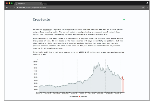
Lesson 2, Model Architecture, shows how to predict Bitcoin prices using deep learning model.

Lesson 3, Model Evaluation and Optimization, shows on how to evaluate a neural network model. We will modify the network’s hyperparameters to improve its performance.

Lesson 4, Productization explains how to productize a deep learning model and also provides an exercise of how to deploy a model as a web application.

Chapter 1. Introduction to Neural Networks and Deep Learning

What are Neural Networks?

Neural networks—also known as Artificial Neural Networks—were first proposed in the 40s by MIT professors Warren McCullough and Walter Pitts.

For more information refer, Explained: Neural networks. MIT News Office, April 14, 2017. Available at: http://news.mit.edu/2017/explained-neural-networks-deep-learning-0414.

Successful Applications

Translating text: In 2017, Google announced that it was releasing a new algorithm for its translation service called Transformer. The algorithm consisted of a recurrent neural network (LSTM) that is trained used bilingual text. Google showed that its algorithm had gained notable accuracy when comparing to industry standards (BLEU) and was also computationally efficient.

Google Research Blog. Transformer: A Novel Neural Network Architecture for Language Understanding. August 31, 2017. Available at: https://research.googleblog.com/2017/08/transformer-novel-neural-network.html.

Self-driving vehicles: Uber, NVIDIA, and Waymo are believed to be using deep learning models to control different vehicle functions that control driving.

Alexis C. Madrigal: Inside Waymo’s Secret World for Training Se Driving Cars. The Atlantic. August 23, 2017. Available https://www.theatlantic.com/technology/archive/2017/08/inside-waymos-secret-testing-and-simulation-
facilities/537648/“>lities/537648/.
NVIDIA: End-to-End Deep Learning for Self-Driving Cars. Augu 17, 2016. Available https://devblogs.nvidia.com/parallelforall/deep-learning-self-driving-cars/.
Dave Gershgorn: Uber’s new AI team is looking for the shorte route to self-driving cars. Quartz. December 5, 2016. Available https://qz.com/853236/ubers-new-ai-team-is-looking-for-the-shortest-route-to-self-driving-cars/.

Image recognition: Facebook and Google use deep learning models to identify entities in images and automatically tag these entities as persons from a set of contacts.

Why Do Neural Networks Work So Well?

Neural networks are powerful because they can be used to predict any given function with reasonable approximation. If one is able to represent a problem as a mathematical function and also has data that represents that function correctly, then a deep learning model can, in principle—and given enough resources—be able to approximate that function. This is typically called the universality principle of neural networks.

For more information refer, Michael Nielsen: Neural Networks and Deep Learning: A visual proof that neural nets can compute any function. Available at: http://neuralnetworksanddeeplearning.com/chap4.html.

Representation Learning

neural networks are computation graphs in which each step computes higher abstraction representations from input data.

Each one of these steps represents a progression into a different abstraction layer. Data progresses through these layers, building continuously higher-level representations. The process finishes with the highest representation possible: the one the model is trying to predict.

Function Approximation

When neural networks learn new representations of data, they do so by combining weights and biases with neurons from different layers.

However, there are many reasons why a neural network may not be able to predict a function with perfection, chief among them being that:

Many functions contain stochastic properties (that is, random properties)
There may be overfitting to peculiarities from the training data
There may be a lack of training data

Limitations of Deep Learning

Deep learning techniques are best suited to problems that can be defined with formal mathematical rules (that is, as data representations). If a problem is hard to define this way, then it is likely that deep learning will not provide a useful solution.

Remember that deep learning algorithms are learning different representations of data to approximate a given function. If data does not represent a function appropriately, it is likely that a function will be incorrectly represented by a neural network.

To avoid this problem, make sure that the data used to train a model represents the problem the model is trying to address as accurately as possible.

Inherent Bias and Ethical Considerations

Researchers have suggested that the use of the deep learning model without considering the inherent bias in the training data can lead not only to poor performing solutions, but also to ethical complications.

Common Components and Operations of Neural Networks

Neural networks have two key components: layers and nodes.
Nodes are responsible for specific operations, and layers are groups of nodes used to differentiate different stages of the system.节点负责特定的操作，而层是用来区分系统不同阶段的节点组。

Nodes are where data is represented in the network. There are two values associated with nodes: biases and weights. Both of these values affect how data is represented by the nodes and passed on to other nodes.

Unfortunately, there isn’t a clear rule for determining how many layers or nodes a network should have.

Configuring a Deep Learning Environment

Activity 1 – Verifying Software Components

函数名	作用	启发
__separator	打印规整的分隔符
test_python	测试 Python 版本是否符合要求
test_tensorflow	测试 TensorFlow 版本是否符合要求	测试其它第三方库时也可以用此方法

def __separator(c):
    """
    Prints a pretty separator.

    Parameters
    ----------
    c: str
        Character to use.
    """
    print(c * 65)

def test_python():
    """
    Tests if Python 3 is installed.
    """
    message = None
    if sys.version_info[0] == 3:
        success = True
        log = """
        PASS: Python 3.0 (or higher) is installed.
        """

    else:
        success = False
        log = """
        FAIL: Python 3.0 (or higher) not detected.
        """
        message = """
            https://www.python.org/downloads/
        """   
    print(log)
    if message:
        print(message)
    __separator('~')
    return success

def test_tensorflow():
    """
    Tests if TensorFlow is installed.
    """
    message = None
    try:
        import tensorflow

        if tensorflow.__version__ >= '1.4.0':
            success = True
            log = """
        PASS: TensorFlow 1.4.0 (or higher) is installed.
            """

        else:
            success = False
            log = """
        FAIL: TensorFlow 1.4.0 (or higher) not detected.
            """
            message = """           
                https://www.tensorflow.org/install/
            """

    except ModuleNotFoundError:
        success = False
        log = """
        FAIL: TensorFlow 1.4.0 (or higher) not detected.
        """
        message = """
                https://www.tensorflow.org/install/
        """  
    print(log)
    if message:
        print(message)

    __separator('~')
    return success

Activity_2_mnist

mnist-demo

Chapter 2. Model Architecture

Older architectures have been used to solve a large array of problems and are generally considered the right choice when starting a new project. Newer architectures have shown great successes in specific problems, but are harder to generalize. The latter are interesting as references of what to explore next, but are hardly a good choice when starting a project.

Choosing the Right Model Architecture

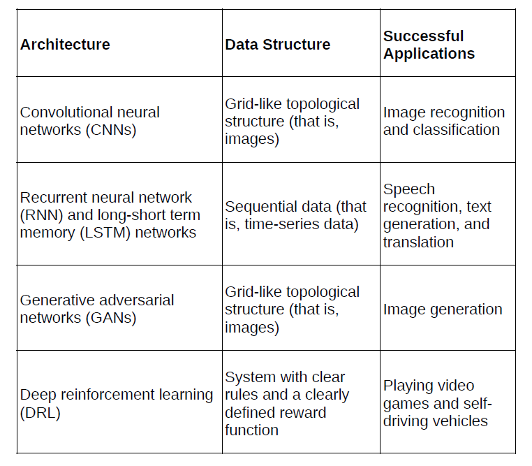
Table 1: Different neural network architectures have shown success in
different fields. The networks’ architecture is typically related to the

Data Normalization

Before building a deep learning model, one more step is necessary: data normalization.

Data normalization is a common practice in machine learning systems. Particularly regarding neural networks, researchers have proposed that normalization is an essential technique for training RNNs (and LSTMs), mainly because it decreases the network’s training time and increases the network’s overall performance.

For more information refer, Batch Normalization: Accelerating Deep Network Training by Reducing Internal Covariate Shift by Sergey Ioffe et. al., arXiv, March 2015. Available at: https://arxiv.org/abs/1502.03167.

Z-score

When data is normally distributed (that is, Gaussian), one can compute the distance between each observation as a standard deviation from its mean. This normalization is useful when identifying how distant data points are from more likely occurrences in the distribution. The Z-score is defined by:

$Z_i=\dfrac{x_i-\mu}{\sigma}$

Here, $x_i$ is the $i^{th}$ observation, $\mu$ is the mean, and $\sigma$ is the stand deviation of the series.

Point-Relative Normalization

This normalization computes the difference of a given observation in relation to the first observation of the series. This kind of normalization is useful to identify trends in relation to a starting point. The point-relative normalization is defined by:

$n_i=(\dfrac{O_i}{O_o})-1$

Here, $O_i$ is the $i^{th}$ observation, $O_o$ is the first observation of the series.

Maximum and Minimum Normalization

This normalization computes the distance between a given observation and the maximum and minimum values of the series. This normalization is useful when working with series in which the maximum and minimum values are not outliers and are important for future predictions. This normalization technique can be applied with:

$n_i=\dfrac{O_i - min(O}{max(O)-min(O}$

Here, $O_i$ is the $i^{th}$ observation,ation, $O$ represents a vector with all $O$ values, and the functions $min(O)$ and $max(O)$ represent the minimum and maximum values of the series, respectively.

Structuring Your Problem

Compared to researchers, practitioners spend much less time determining which architecture to choose when starting a new deep learning project. Acquiring data that represents a given problem correctly is the most important factor to consider when developing these systems, followed by the understanding of the dataset’s inherent biases and limitations.

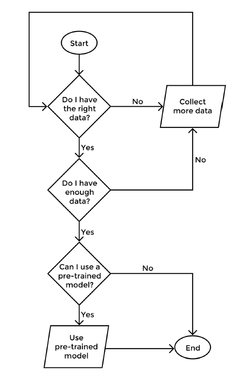
Figure 5: Decision-tree of key reflection questions to be made at the beginning of a deep learning project

Activity 3 – Exploring the Bitcoin Dataset and Preparing Data for Model

1	bitcoin = pd.read_csv('data/bitcoin_historical_prices.csv')

Our dataset contains 7 variables (i.e. columns). Here’s what each one of them represents:

date: date of the observation.
iso_week: week number of a given year.
open: open value of a single Bitcoin coin.
high: highest value achieved during a given day period.
low: lowest value achieved during a given day period.
close: value at the close of the transaction day.
volume: what is the total volume of Bitcoin that was exchanged during that day.
market_capitalization: as described in CoinMarketCap’s FAQ page, this is calculated by Market Cap = Price X Circulating Supply.

All values are in USD.

Exploration

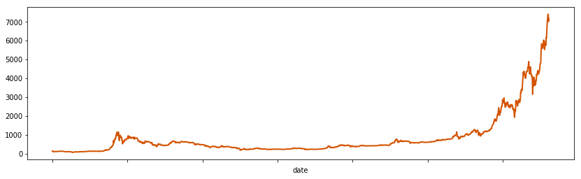
We will now explore the dataset timeseries to understand its patterns.

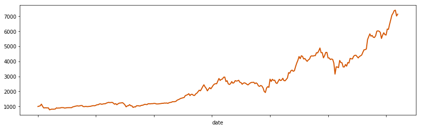
Let’s first explore two variables: close price and volume. Volume only contains data starting in November 2013, while close prices start earlier in April of that year. However, both show similar spiking patterns starting at the beginning of 2017.

1	bitcoin.set_index('date')['close'].plot(linewidth=2, figsize=(14, 4), color='#d35400')

<matplotlib.axes._subplots.AxesSubplot at 0x8869048>

Now let’s explore the yera of 2017 only. This is the year where the price of bitcoin has risen significantly.

1 2	bitcoin[bitcoin['date'] >= '2017-01-01'].set_index('date')['close'].plot( linewidth=2, figsize=(14, 4), color='#d35400')

<matplotlib.axes._subplots.AxesSubplot at 0x8b50048>

Preparing Dataset for Model

Neural networks typically work with either matrices) or tensors. Our data needs to fit that structure before it can be used by either keras (or tensorflow).

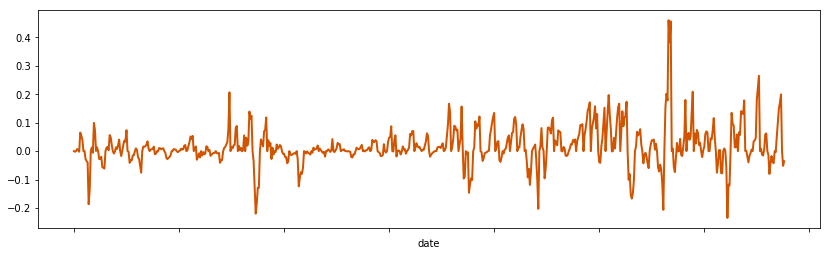
Also, it is common practice to normalize data before using it to train a neural network. We will be using a normalization technique the evaluates each observation into a range between 0 and 1 in relation to the first observation in each week.

1	bitcoin.head()

	date	iso_week	open	high	low	close	volume	market_capitalization
0	2013-04-28	2013-17	135.30	135.98	132.10	134.21	NaN	1.500520e+09
1	2013-04-29	2013-17	134.44	147.49	134.00	144.54	NaN	1.491160e+09
2	2013-04-30	2013-17	144.00	146.93	134.05	139.00	NaN	1.597780e+09
3	2013-05-01	2013-17	139.00	139.89	107.72	116.99	NaN	1.542820e+09
4	2013-05-02	2013-17	116.38	125.60	92.28	105.21	NaN	1.292190e+09

First, let’s remove data from older periods. We will keep only data from 2016 until the latest observation of 2017. Older observations may be useful to understand current prices. However, Bitcoin has gained so much popularity in recent years that including older data would require a more laborious treatment. We will leave that for a future exploration.

1	bitcoin_recent = bitcoin[bitcoin['date'] >= '2016-01-01']

Let’s keep only the close and volume variables. We can use the other variables in another time.

1	bitcoin_recent = bitcoin_recent[['date', 'iso_week', 'close', 'volume']]

Now, let’s normalize our data for both the close and volume variables.

1 2	bitcoin_recent['close_point_relative_normalization'] = bitcoin_recent.groupby('iso_week')['close'].apply( lambda x: normalizations.point_relative_normalization(x))

1 2	bitcoin_recent.set_index('date')['close_point_relative_normalization'].plot( linewidth=2, figsize=(14, 4), color='#d35400')

<matplotlib.axes._subplots.AxesSubplot at 0xb81d160>

Using Keras as a TensorFlow Interface

Keras simplifies the interface for working with different architectures by using three components - network architecture, fit, and predict:

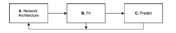
Figure 15: The Keras neural network paradigm: A. design a neural network architecture, B. Train a neural network (or Fit), and C. Make predictions

Activity 4 – Creating a TensorFlow Model Using Keras

# build_model
model = Sequential()
model.add(LSTM(
    units=period_length,
    batch_input_shape=(batch_size, number_of_periods, period_length),
    input_shape=(number_of_periods, period_length),
    return_sequences=False, stateful=False))

model.add(Dense(units=period_length))
model.add(Activation("linear"))

model.compile(loss="mse", optimizer="rmsprop")
## saving model
model.save('bitcoin_lstm_v0.h5')

Activity 5 – Assembling a Deep Learning System

# Shaping Data
X_train = data[:-1,:].reshape(1, 76, 7)
Y_validation = data[-1].reshape(1, 7)
# Load Model
model = load_model('bitcoin_lstm_v0.h5')
# Make Predictions
%%time
history = model.fit(x=X_train, y=Y_validation,
                    batch_size=32, epochs=100)

Chapter 3. Model Evaluation and Optimization

Parameter and Hyperparameter

Parameters are properties that affect how a model makes predictions from data. Hyperparameters refer to how a model learns from data. Parameters can be learned from the data and modified dynamically. Hyperparameters are higher-level properties and are not typically learned from data.

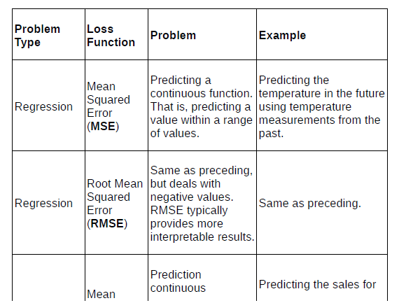
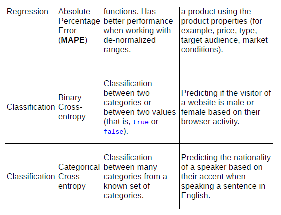
Table 1: Common loss functions used for classification and regression problems

We learned that loss functions are key elements of neural networks, as they evaluate the performance of a network at each epoch and are the starting point for the propagation of adjustments back into layers and nodes. We also explored why some loss functions can be difficult to interpret (for instance, the MSE) and developed a strategy using two other functions—RMSE and MAPE—to interpret the predicted results from our LSTM model.

Activity 6 – Creating an Active Training Environment

Layers and Nodes - Adding More Layers

the more layers you add, the more hyperparameters you have to tune—and the longer your network will take to train. If your model is performing fairly well and not overfitting your data, experiment with the other strategies outlined in this lesson before adding new layers to your network.

Epochs

he larger the date used to train your model, the more epochs it will need to achieve good performance.

Activation Functions

Understanding Activation Functions in Neural Networks by Avinash Sharma V, available at: https://medium.com/the-theory-of-everything/understanding-activation-functions-in-neural-networks-9491262884e0.

L2 Regularization

L2 regularization (or weight decay) is a common technique for dealing with overfitting models. In some models, certain parameters vary in great magnitudes. The L2 regularization penalizes such parameters, reducing the effect of these parameters on the network.

Dropout

Dropout is a regularization technique based on a simple question: if one randomly takes away a proportion of nodes from layers, how will the other node adapt? It turns out that the remaining neurons adapt, learning to represent patterns that were previously handled by those neurons that are missing.

Activity 7: Optimizing a deep learning model

# 使用 tensorboard 辅助训练的函数
def train_model(model, X, Y, epochs=100, version=0, run_number=0):
    """
    Shorthand function for training a new model.
    This function names each run of the model
    using the TensorBoard naming conventions.

    Parameters
    ----------
    model: Keras model instance
        Compiled Keras model.
    X, Y: np.array
        Series of observations to be used in
        the training process.
    version: int
        Version of the model to run.
    run_number: int
        The number of the run. Used in case
        the same model version is run again.
    """
    hash = random.getrandbits(128)
    hex_code = '%032x' % hash
    model_name = 'bitcoin_lstm_v{version}_run_{run_number}_{hex_code}'.format(
        version=version, run_number=run_number, hex_code=hex_code[:6])

    tensorboard = TensorBoard(log_dir='./logs/{}'.format(model_name))

    model_history = model.fit(
        x=X, y=Y,
        batch_size=1, epochs=epochs,
        verbose=0, callbacks=[tensorboard],
        shuffle=False)

    return model_history

Chapter 4. Productization

This lesson focuses on how to productize a deep learning model. We use the word productize to define the creation of a software product from a deep learning model that can be used by other people and applications.
We are interested in models that use new data when it becomes available, continuously learning patterns from new data and, consequently, making better predictions. We study two strategies to deal with new data: one that re-trains an existing model, and another that creates a completely new model. Then, we implement the latter strategy in our Bitcoin prices prediction model so that it can continuously predict new Bitcoin prices.

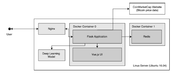
Figure 1: System architecture for the web application built in this project

Handling New Data

Models can be trained once in a set of data and can then be used to make predictions. Such static models can be very useful, but it is often the case that we want our model to continuously learn from new data—and to continuously get better as it does so.
In this section, we will discuss two strategies on how to re-train a deep learning model and how to implement them in Python.

Separating Data and Model

When building a deep learning application, the two most important areas are data and model. From an architectural point of view, we suggest that these two areas be separate. We believe that is a good suggestion because each of these areas include functions inherently separated from each other. Data is often required to be collected, cleaned, organized, and normalized; and models need to be trained, evaluated, and able to make predictions. Both of these areas are dependent, but are better dealt with separately.
As a matter of following that suggestion, we will be using two classes to help us build our web application: CoinMarketCap() and Model():

CoinMarketCap(): This is a class designed for fetching Bitcoin prices from the following website: http://www.coinmarketcap.com. This is the same place where our original Bitcoin data comes from. This class makes it easy to retrieve that data on a regular schedule, returning a Pandas DataFrame with the parsed records and all available historical data.
Model(): This class implements all the code we have written so far into a single class. That class provides facilities for interacting with our previously trained models, and also allows for the making of predictions using de-normalized data—which is much easier to understand. The Model() class is our model component.

These two classes are used extensively throughout our example application and define the data and model components.

前言