0%

支持向量机

经典支持向量机 Support Vector Machines

在机器学习中,支持向量机是在分类与回归分析中分析数据的监督式学习模型与相关的学习算法。给定一组训练实例,每个训练实例被标记为属于两个类别中的一个或另一个,SVM训练算法创建一个将新的实例分配给两个类别之一的模型,使其成为非概率二元线性分类器。SVM模型是将实例表示为空间中的点,这样映射就使得单独类别的实例被尽可能宽的明显的间隔分开。然后,将新的实例映射到同一空间,并基于它们落在间隔的哪一侧来预测所属类别。

个人建议学习支持向量机的方法:

  1. 熟读理论 支持向量机通俗导论(理解SVM的三层境界)LaTeX最新版_2015.1.9 PDF
  2. 应用支持向量机解决实际问题

支持向量机资源

点到直线距离公式

Support Vector Machines

This chapter shows how to implement various SVM methods with TensorFlow. We first create a linear SVM and also show how it can be used for regression. We then introduce kernels (RBF Gaussian kernel) and show how to use it to split up non-linear data. We finish with a multi-dimensional implementation of non-linear SVMs to work with multiple classes.

1. Linear Support Vector Machine: Soft Margin

Model
We will aim to maximize the margin width, 2/||A||, or minimize ||A||. We allow for a soft margin by having an error term in the loss function which is the max(0, 1-pred*actual).

Linear Separator

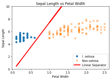
This function shows how to use TensorFlow to create a soft margin SVM
We will use the iris data, specifically:

$x_1 =$ Sepal Length

$x_2 =$ Petal Width

Class 1 : I. setosa

Class -1: not I. setosa

We know here that x and y are linearly seperable for I. setosa classification.

Note that we implement the soft margin with an allowable margin of error for points. The margin of error term is given by ‘alpha’ below. To behave like a hard margin SVM, set alpha = 0. (in notebook code block #7)

1
2
3
4
5
6
import matplotlib.pyplot as plt
import numpy as np
import tensorflow as tf
from sklearn import datasets
from tensorflow.python.framework import ops
ops.reset_default_graph()

Set a random seed and start a computational graph.

1
2
3
np.random.seed(41)
tf.set_random_seed(41)
sess = tf.Session()

Load the data

1
2
3
4
# iris.data = [(Sepal Length, Sepal Width, Petal Length, Petal Width)]
iris = datasets.load_iris()
x_vals = np.array([[x[0], x[3]] for x in iris.data])
y_vals = np.array([1 if y == 0 else -1 for y in iris.target])

Split data into train/test sets

1
2
3
4
5
6
train_indices = np.random.choice(len(x_vals), round(len(x_vals)*0.8), replace=False)
test_indices = np.array(list(set(range(len(x_vals))) - set(train_indices)))
x_vals_train = x_vals[train_indices]
x_vals_test = x_vals[test_indices]
y_vals_train = y_vals[train_indices]
y_vals_test = y_vals[test_indices]

Set model parameters, placeholders, and coefficients.

1
2
3
4
5
6
7
8
9
10
# Declare batch size
batch_size = 110

# Initialize placeholders
x_data = tf.placeholder(shape=[None, 2], dtype=tf.float32)
y_target = tf.placeholder(shape=[None, 1], dtype=tf.float32)

# Create variables for SVM
A = tf.Variable(tf.random_normal(shape=[2, 1]))
b = tf.Variable(tf.random_normal(shape=[1, 1]))

Declare our model and L2 Norm

SVM linear model is given by the equation:

Our loss function will be the above quantity and we will tell TensorFlow to minimize it. Note that $n$ is the number of points (in a batch), $A$ is the hyperplane-normal vector (to solve for), $b$ is the hyperplane-offset (to solve for), and $\alpha$ is the soft-margin parameter.

1
2
3
4
5
# Declare model operations
model_output = tf.subtract(tf.matmul(x_data, A), b)

# Declare vector L2 'norm' function squared
l2_norm = tf.reduce_sum(tf.square(A))

Here we make our special loss function based on the classification of the points (which side of the line they fall on).

Also, note that alpha is the soft-margin term and an be increased to allow for more erroroneous classification points. For hard-margin behaviour, set alpha = 0.

1
2
3
4
5
6
7
8
9
10
11
# Declare loss function
# Loss = max(0, 1-pred*actual) + alpha * L2_norm(A)^2
# L2 regularization parameter, alpha

alpha = tf.constant([0.01])

# Margin term in loss
classification_term = tf.reduce_mean(tf.maximum(0., tf.subtract(1., tf.multiply(model_output, y_target))))

# Put terms together
loss = tf.add(classification_term, tf.multiply(alpha, l2_norm))

Creat the prediction function, optimization algorithm, and initialize the variables.

1
2
3
4
5
6
7
8
9
10
11
# Declare prediction function
prediction = tf.sign(model_output)
accuracy = tf.reduce_mean(tf.cast(tf.equal(prediction, y_target), tf.float32))

# Declare optimizer
my_opt = tf.train.AdamOptimizer(0.005)
train_step = my_opt.minimize(loss)

# Initialize variables
init = tf.global_variables_initializer()
sess.run(init)

Now we can start the training loop.

1
2
3
4
5
6
7
8
9
10
11
12
13
14
15
16
17
18
19
20
21
22
23
24
25
26
27
28
29
30
# Training loop
loss_vec = []
train_accuracy = []
test_accuracy = []
for i in range(1500):
rand_index = np.random.choice(len(x_vals_train), size=batch_size)
rand_x = x_vals_train[rand_index]
rand_y = np.transpose([y_vals_train[rand_index]])
sess.run(train_step, feed_dict={x_data: rand_x, y_target: rand_y})

temp_loss = sess.run(loss, feed_dict={x_data: rand_x, y_target: rand_y})
loss_vec.append(temp_loss)

train_acc_temp = sess.run(accuracy, feed_dict={
x_data: x_vals_train,
y_target: np.transpose([y_vals_train])})
train_accuracy.append(train_acc_temp)

test_acc_temp = sess.run(accuracy, feed_dict={
x_data: x_vals_test,
y_target: np.transpose([y_vals_test])})
test_accuracy.append(test_acc_temp)

if (i + 1) % 75 == 0:
print('Step #{} A = {}, b = {}'.format(
str(i+1),
str(sess.run(A)),
str(sess.run(b))
))
print('Loss = ' + str(temp_loss))
Step #75 A = [[0.65587175]
 [0.73911524]], b = [[0.8189382]]
Loss = [3.477592]
Step #150 A = [[0.30820864]
 [0.37043768]], b = [[1.1588708]]
Loss = [1.8782018]
Step #225 A = [[0.05466489]
 [0.01620324]], b = [[1.3756151]]
Loss = [0.61904156]
Step #300 A = [[ 0.0723089 ]
 [-0.10384972]], b = [[1.2969997]]
Loss = [0.50430346]
Step #375 A = [[ 0.08872697]
 [-0.21590038]], b = [[1.214785]]
Loss = [0.5581]
Step #450 A = [[ 0.10302152]
 [-0.33577552]], b = [[1.1402861]]
Loss = [0.60070616]
Step #525 A = [[ 0.12028296]
 [-0.46366042]], b = [[1.0620526]]
Loss = [0.47809908]
Step #600 A = [[ 0.145114 ]
 [-0.5994784]], b = [[0.97037107]]
Loss = [0.56837624]
Step #675 A = [[ 0.16354088]
 [-0.7458743 ]], b = [[0.8814289]]
Loss = [0.5452542]
Step #750 A = [[ 0.17879468]
 [-0.90772235]], b = [[0.7907687]]
Loss = [0.47175956]
Step #825 A = [[ 0.20936723]
 [-1.0691159 ]], b = [[0.68023866]]
Loss = [0.41458404]
Step #900 A = [[ 0.236106 ]
 [-1.2391785]], b = [[0.5687398]]
Loss = [0.29367676]
Step #975 A = [[ 0.25400215]
 [-1.4175524 ]], b = [[0.46441486]]
Loss = [0.27020118]
Step #1050 A = [[ 0.28435734]
 [-1.5984066 ]], b = [[0.34036276]]
Loss = [0.19518965]
Step #1125 A = [[ 0.28947413]
 [-1.780023  ]], b = [[0.24134117]]
Loss = [0.17559259]
Step #1200 A = [[ 0.2927576]
 [-1.930816 ]], b = [[0.15315719]]
Loss = [0.13242653]
Step #1275 A = [[ 0.3031533]
 [-2.0399208]], b = [[0.06639722]]
Loss = [0.14762701]
Step #1350 A = [[ 0.29892927]
 [-2.1220415 ]], b = [[0.00746888]]
Loss = [0.1029826]
Step #1425 A = [[ 0.29492435]
 [-2.1905353 ]], b = [[-0.04703728]]
Loss = [0.11851373]
Step #1500 A = [[ 0.29012206]
 [-2.2488031 ]], b = [[-0.09580647]]
Loss = [0.1065909]

Now we extract the linear coefficients and get the SVM boundary line.

1
2
3
4
5
6
7
8
9
10
11
12
13
14
15
16
17
18
19
# Extract coefficients
[[a1], [a2]] = sess.run(A)
[[b]] = sess.run(b)
slope = -a2/a1
y_intercept = b/a1

# Extract x1 and x2 vals
x1_vals = [d[1] for d in x_vals]

# Get best fit line
best_fit = []
for i in x1_vals:
best_fit.append(slope*i+y_intercept)

# Separate I. setosa
setosa_x = [d[1] for i, d in enumerate(x_vals) if y_vals[i] == 1]
setosa_y = [d[0] for i, d in enumerate(x_vals) if y_vals[i] == 1]
not_setosa_x = [d[1] for i, d in enumerate(x_vals) if y_vals[i] == -1]
not_setosa_y = [d[0] for i, d in enumerate(x_vals) if y_vals[i] == -1]

Matplotlib code for plotting

$a_1x_1 + a_2x_2 - b = 0$

$x_1 =$ Sepal Length

$x_2 =$ Petal Width

1
2
3
4
5
6
7
8
9
10
11
12
13
14
15
16
17
18
19
20
21
22
23
24
25
26
27
%matplotlib inline
# Plot data and line
plt.plot(setosa_x, setosa_y, 'o', label='I. setosa')
plt.plot(not_setosa_x, not_setosa_y, 'x', label='Non-setosa')
plt.plot(x1_vals, best_fit, 'r-', label='Linear Separator', linewidth=3)
plt.ylim([0, 10])
plt.legend(loc='lower right')
plt.title('Sepal Length vs Petal Width')
plt.xlabel('Petal Width')
plt.ylabel('Sepal Length')
plt.show()

# Plot train/test accuracies
plt.plot(train_accuracy, 'k-', label='Training Accuracy')
plt.plot(test_accuracy, 'r--', label='Test Accuracy')
plt.title('Train and Test Set Accuracies')
plt.xlabel('Generation')
plt.ylabel('Accuracy')
plt.legend(loc='lower right')
plt.show()

# Plot loss over time
plt.plot(loss_vec, 'k-')
plt.title('Loss per Generation')
plt.xlabel('Generation')
plt.ylabel('Loss')
plt.show()

png
png
png


2. SVM Regression

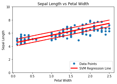
This function shows how to use TensorFlow to solve support vector regression. We are going
to find the line that has the maximum margin which INCLUDES as many points as possible.

We will use the iris data, specifically:

$y =$ Sepal Length

$x =$ Pedal Width

To start, load the necessary libraries:

1
2
3
4
5
6
import matplotlib.pyplot as plt
import numpy as np
import tensorflow as tf
from sklearn import datasets
from tensorflow.python.framework import ops
ops.reset_default_graph()

Create a TF Graph Session:

1
sess = tf.Session()

Load the iris data, use the Sepal Length and Petal width for SVM regression.

1
2
3
4
5
6
7
8
9
10
11
12
13
# Load the data
# iris.data = [(Sepal Length, Sepal Width, Petal Length, Petal Width)]
iris = datasets.load_iris()
x_vals = np.array([x[3] for x in iris.data])
y_vals = np.array([y[0] for y in iris.data])

# Split data into train/test sets
train_indices = np.random.choice(len(x_vals), round(len(x_vals)*0.8), replace=False)
test_indices = np.array(list(set(range(len(x_vals))) - set(train_indices)))
x_vals_train = x_vals[train_indices]
x_vals_test = x_vals[test_indices]
y_vals_train = y_vals[train_indices]
y_vals_test = y_vals[test_indices]

Declare the batch size, initialize placeholders, and create linear regression variables

1
2
3
4
5
6
7
8
9
10
# Declare batch size
batch_size = 50

# Initialize placeholders
x_data = tf.placeholder(shape=[None, 1], dtype=tf.float32)
y_target = tf.placeholder(shape=[None, 1], dtype=tf.float32)

# Create variables for linear regression
A = tf.Variable(tf.random_normal(shape=[1,1]))
b = tf.Variable(tf.random_normal(shape=[1,1]))

Create the model

1
2
# Declare model operations
model_output = tf.add(tf.matmul(x_data, A), b)

Our loss function, which maximizes the amount of points near the line.

1
2
3
4
5
6
# Declare loss function
# = max(0, abs(target - predicted) + epsilon)
# 1/2 margin width parameter = epsilon
epsilon = tf.constant([0.5])
# Margin term in loss
loss = tf.reduce_mean(tf.maximum(0., tf.subtract(tf.abs(tf.subtract(model_output, y_target)), epsilon)))

Create the optimization function and initialize all the model variables

1
2
3
4
5
6
7
# Declare optimizer
my_opt = tf.train.GradientDescentOptimizer(0.075)
train_step = my_opt.minimize(loss)

# Initialize variables
init = tf.global_variables_initializer()
sess.run(init)

Train! Loop through batches of data and optimize.

1
2
3
4
5
6
7
8
9
10
11
12
13
14
15
16
17
18
19
20
# Training loop
train_loss = []
test_loss = []
for i in range(200):
rand_index = np.random.choice(len(x_vals_train), size=batch_size)
rand_x = np.transpose([x_vals_train[rand_index]])
rand_y = np.transpose([y_vals_train[rand_index]])
sess.run(train_step, feed_dict={x_data: rand_x, y_target: rand_y})

temp_train_loss = sess.run(loss, feed_dict={x_data: np.transpose([x_vals_train]), y_target: np.transpose([y_vals_train])})
train_loss.append(temp_train_loss)

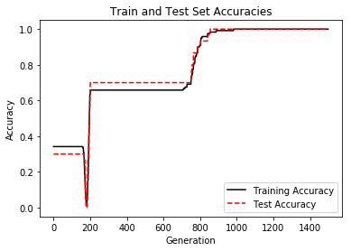
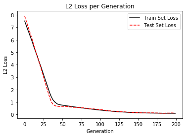
temp_test_loss = sess.run(loss, feed_dict={x_data: np.transpose([x_vals_test]), y_target: np.transpose([y_vals_test])})
test_loss.append(temp_test_loss)
if (i+1)%50==0:
print('-----------')
print('Generation: ' + str(i+1))
print('A = ' + str(sess.run(A)) + ' b = ' + str(sess.run(b)))
print('Train Loss = ' + str(temp_train_loss))
print('Test Loss = ' + str(temp_test_loss))
-----------
Generation: 50
A = [[2.4289258]] b = [[2.271079]]
Train Loss = 0.7553672
Test Loss = 0.65542704
-----------
Generation: 100
A = [[1.9204257]] b = [[3.4155781]]
Train Loss = 0.3573223
Test Loss = 0.39466858
-----------
Generation: 150
A = [[1.3823755]] b = [[4.095077]]
Train Loss = 0.14115657
Test Loss = 0.14801341
-----------
Generation: 200
A = [[1.204475]] b = [[4.462577]]
Train Loss = 0.09575871
Test Loss = 0.11255897

For plotting, we need to extract the coefficients and get the best fit line. (Also the upper and lower margins.)

1
2
3
4
5
6
7
8
9
10
11
12
13
# Extract Coefficients
[[slope]] = sess.run(A)
[[y_intercept]] = sess.run(b)
[width] = sess.run(epsilon)

# Get best fit line
best_fit = []
best_fit_upper = []
best_fit_lower = []
for i in x_vals:
best_fit.append(slope*i+y_intercept)
best_fit_upper.append(slope*i+y_intercept+width)
best_fit_lower.append(slope*i+y_intercept-width)

Matplotlib code to plot the fit and loss.

1
2
3
4
5
6
7
8
9
10
11
12
13
14
15
16
17
18
19
20
# Plot fit with data
plt.plot(x_vals, y_vals, 'o', label='Data Points')
plt.plot(x_vals, best_fit, 'r-', label='SVM Regression Line', linewidth=3)
plt.plot(x_vals, best_fit_upper, 'r--', linewidth=2)
plt.plot(x_vals, best_fit_lower, 'r--', linewidth=2)
plt.ylim([0, 10])
plt.legend(loc='lower right')
plt.title('Sepal Length vs Petal Width')
plt.xlabel('Petal Width')
plt.ylabel('Sepal Length')
plt.show()

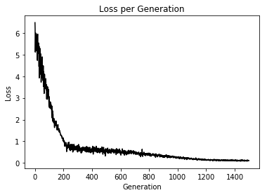
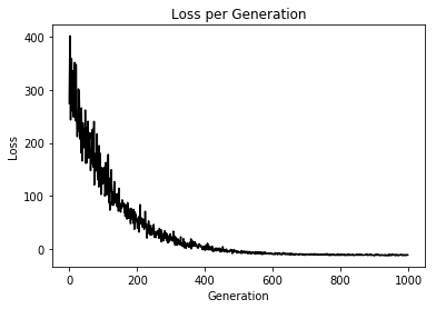
# Plot loss over time
plt.plot(train_loss, 'k-', label='Train Set Loss')
plt.plot(test_loss, 'r--', label='Test Set Loss')
plt.title('L2 Loss per Generation')
plt.xlabel('Generation')
plt.ylabel('L2 Loss')
plt.legend(loc='upper right')
plt.show()

png
png


3. Illustration of Various Kernels

Working with Kernels

Linear SVMs are very powerful. But sometimes the data are not very linear. To this end, we can use the ‘kernel trick’ to map our data into a higher dimensional space, where it may be linearly separable. Doing this allows us to separate out non-linear classes. See the below example.

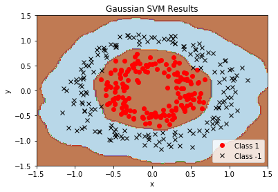
If we attempt to separate the below circular-ring shaped classes with a standard linear SVM, we fail.

Linear SVM Nonlinear Data

But if we separate it with a Gaussian-RBF kernel, we can find a linear separator in a higher dimension that works a lot better.

Gaussian Kernel Nonlinear Data

This function wll illustrate how to implement various kernels in TensorFlow.

Linear Kernel:

Gaussian Kernel (RBF):

We start by loading the necessary libraries

1
2
3
4
5
6
import matplotlib.pyplot as plt
import numpy as np
import tensorflow as tf
from sklearn import datasets
from tensorflow.python.framework import ops
ops.reset_default_graph()

Start a computational graph session:

1
sess = tf.Session()

For this example, we will generate fake non-linear data. The data we will generate is concentric ring data.

1
2
3
4
5
6
7
# Generate non-lnear data
(x_vals, y_vals) = datasets.make_circles(n_samples=350, factor=.5, noise=.1)
y_vals = np.array([1 if y==1 else -1 for y in y_vals])
class1_x = [x[0] for i,x in enumerate(x_vals) if y_vals[i]==1]
class1_y = [x[1] for i,x in enumerate(x_vals) if y_vals[i]==1]
class2_x = [x[0] for i,x in enumerate(x_vals) if y_vals[i]==-1]
class2_y = [x[1] for i,x in enumerate(x_vals) if y_vals[i]==-1]

We declare the batch size (large for SVMs), create the placeholders, and declare the $b$ variable for the SVM model.

1
2
3
4
5
6
7
8
9
10
# Declare batch size
batch_size = 350

# Initialize placeholders
x_data = tf.placeholder(shape=[None, 2], dtype=tf.float32)
y_target = tf.placeholder(shape=[None, 1], dtype=tf.float32)
prediction_grid = tf.placeholder(shape=[None, 2], dtype=tf.float32)

# Create variables for svm
b = tf.Variable(tf.random_normal(shape=[1,batch_size]))

Here we will apply the kernel. Note that the Linear Kernel is commented out. If you choose to use the linear kernel, then uncomment the linear my_kernel variable, and comment out the five RBF kernel lines.

1
2
3
4
5
6
7
8
9
10
# Apply kernel
# Linear Kernel
# my_kernel = tf.matmul(x_data, tf.transpose(x_data))

# Gaussian (RBF) kernel
gamma = tf.constant(-50.0)
dist = tf.reduce_sum(tf.square(x_data), 1)
dist = tf.reshape(dist, [-1,1])
sq_dists = tf.add(tf.subtract(dist, tf.multiply(2., tf.matmul(x_data, tf.transpose(x_data)))), tf.transpose(dist))
my_kernel = tf.exp(tf.multiply(gamma, tf.abs(sq_dists)))

Next we compute the SVM model and create a loss function.

1
2
3
4
5
6
# Compute SVM Model
first_term = tf.reduce_sum(b)
b_vec_cross = tf.matmul(tf.transpose(b), b)
y_target_cross = tf.matmul(y_target, tf.transpose(y_target))
second_term = tf.reduce_sum(tf.multiply(my_kernel, tf.multiply(b_vec_cross, y_target_cross)))
loss = tf.negative(tf.subtract(first_term, second_term))

Just like we created the kernel for the training points, we need to create the kernel for the test/prediction points.

Again, comment/uncomment the appropriate lines for using the linear or RBF kernel.

1
2
3
4
5
6
7
8
9
# Create Prediction Kernel
# Linear prediction kernel
# my_kernel = tf.matmul(x_data, tf.transpose(prediction_grid))

# Gaussian (RBF) prediction kernel
rA = tf.reshape(tf.reduce_sum(tf.square(x_data), 1),[-1,1])
rB = tf.reshape(tf.reduce_sum(tf.square(prediction_grid), 1),[-1,1])
pred_sq_dist = tf.add(tf.subtract(rA, tf.multiply(2., tf.matmul(x_data, tf.transpose(prediction_grid)))), tf.transpose(rB))
pred_kernel = tf.exp(tf.multiply(gamma, tf.abs(pred_sq_dist)))

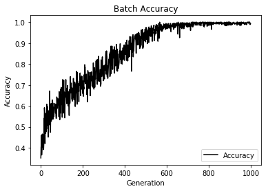
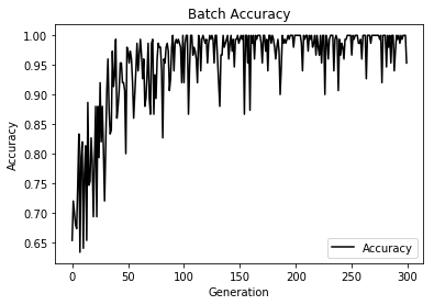
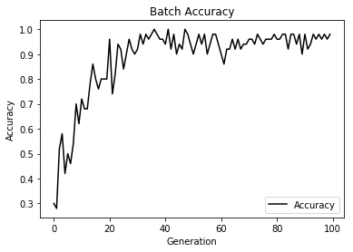
In order to use the kernel to classify points, we create a prediction operation. This prediction operation will be the sign ( positive or negative ) of the model outputs. The accuracy can then be computed if we know the actual target labels.
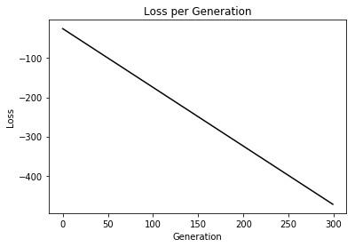
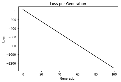
1
2
3
prediction_output = tf.matmul(tf.multiply(tf.transpose(y_target),b), pred_kernel)
prediction = tf.sign(prediction_output-tf.reduce_mean(prediction_output))
accuracy = tf.reduce_mean(tf.cast(tf.equal(tf.squeeze(prediction), tf.squeeze(y_target)), tf.float32))

We now declare the optimizer and variable initialization operations.

1
2
3
4
5
6
7
# Declare optimizer
my_opt = tf.train.GradientDescentOptimizer(0.002)
train_step = my_opt.minimize(loss)

# Initialize variables
init = tf.global_variables_initializer()
sess.run(init)

We start the training loop for the SVM. We will randomly choose a batch of points and run the train step. Then we calculate the loss and accuracy.

1
2
3
4
5
6
7
8
9
10
11
12
13
14
15
16
17
18
19
20
# Training loop
loss_vec = []
batch_accuracy = []
for i in range(1000):
rand_index = np.random.choice(len(x_vals), size=batch_size)
rand_x = x_vals[rand_index]
rand_y = np.transpose([y_vals[rand_index]])
sess.run(train_step, feed_dict={x_data: rand_x, y_target: rand_y})

temp_loss = sess.run(loss, feed_dict={x_data: rand_x, y_target: rand_y})
loss_vec.append(temp_loss)

acc_temp = sess.run(accuracy, feed_dict={x_data: rand_x,
y_target: rand_y,
prediction_grid:rand_x})
batch_accuracy.append(acc_temp)

if (i+1)%250==0:
print('Step #' + str(i+1))
print('Loss = ' + str(temp_loss))
Step #250
Loss = 46.040836
Step #500
Loss = -5.635271
Step #750
Loss = -11.075392
Step #1000
Loss = -11.158321

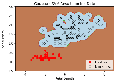
To plot a pretty picture of the regions we fit, we create a fine mesh to run through our model and get the predictions. (This is very similar to the SVM plotting code from sci-kit learn).

1
2
3
4
5
6
7
8
9
10
# Create a mesh to plot points in
x_min, x_max = x_vals[:, 0].min() - 1, x_vals[:, 0].max() + 1
y_min, y_max = x_vals[:, 1].min() - 1, x_vals[:, 1].max() + 1
xx, yy = np.meshgrid(np.arange(x_min, x_max, 0.02),
np.arange(y_min, y_max, 0.02))
grid_points = np.c_[xx.ravel(), yy.ravel()]
[grid_predictions] = sess.run(prediction, feed_dict={x_data: x_vals,
y_target: np.transpose([y_vals]),
prediction_grid: grid_points})
grid_predictions = grid_predictions.reshape(xx.shape)

Plot the results

1
2
3
4
5
6
7
8
9
10
11
12
13
14
15
16
17
18
19
20
21
22
23
24
25
26
# Plot points and grid
plt.contourf(xx, yy, grid_predictions, cmap=plt.cm.Paired, alpha=0.8)
plt.plot(class1_x, class1_y, 'ro', label='Class 1')
plt.plot(class2_x, class2_y, 'kx', label='Class -1')
plt.title('Gaussian SVM Results')
plt.xlabel('x')
plt.ylabel('y')
plt.legend(loc='lower right')
plt.ylim([-1.5, 1.5])
plt.xlim([-1.5, 1.5])
plt.show()

# Plot batch accuracy
plt.plot(batch_accuracy, 'k-', label='Accuracy')
plt.title('Batch Accuracy')
plt.xlabel('Generation')
plt.ylabel('Accuracy')
plt.legend(loc='lower right')
plt.show()

# Plot loss over time
plt.plot(loss_vec, 'k-')
plt.title('Loss per Generation')
plt.xlabel('Generation')
plt.ylabel('Loss')
plt.show()

png
png
png

Prediction/Evaluation

Here is code on how to predict the class on new or unseen data.

1
2
3
4
5
6
7
# New data points:
new_points = np.array([(-0.75, -0.75),
(-0.5, -0.5),
(-0.25, -0.25),
(0.25, 0.25),
(0.5, 0.5),
(0.75, 0.75)])
1
2
3
[evaluations] = sess.run(prediction, feed_dict={x_data: x_vals,
y_target: np.transpose([y_vals]),
prediction_grid: new_points})
1
2
for ix, p in enumerate(new_points):
print('{} : class={}'.format(p, evaluations[ix]))
[-0.75 -0.75] : class=-1.0
[-0.5 -0.5] : class=1.0
[-0.25 -0.25] : class=1.0
[0.25 0.25] : class=1.0
[0.5 0.5] : class=-1.0
[0.75 0.75] : class=-1.0

4. Implementing NonLinear SVMs

Here we show how to use the prior Gaussian RBF kernel to predict I.setosa from the Iris dataset.

Nonlinear SVM

This function wll illustrate how to implement the gaussian kernel on the iris dataset.

Gaussian Kernel:

We start by loading the necessary libraries and resetting the computational graph.

1
2
3
4
5
6
import matplotlib.pyplot as plt
import numpy as np
import tensorflow as tf
from sklearn import datasets
from tensorflow.python.framework import ops
ops.reset_default_graph()

Create a graph session

1
sess = tf.Session()

Load the Iris Data

Our x values will be $(x_1, x_2)$ where,

$x_1 =$ ‘Sepal Length’

$x_2 =$ ‘Petal Width’

The Target values will be wether or not the flower species is Iris Setosa.

1
2
3
4
5
6
7
8
9
# Load the data
# iris.data = [(Sepal Length, Sepal Width, Petal Length, Petal Width)]
iris = datasets.load_iris()
x_vals = np.array([[x[0], x[3]] for x in iris.data])
y_vals = np.array([1 if y==0 else -1 for y in iris.target])
class1_x = [x[0] for i,x in enumerate(x_vals) if y_vals[i]==1]
class1_y = [x[1] for i,x in enumerate(x_vals) if y_vals[i]==1]
class2_x = [x[0] for i,x in enumerate(x_vals) if y_vals[i]==-1]
class2_y = [x[1] for i,x in enumerate(x_vals) if y_vals[i]==-1]

Model Parameters

We now declare our batch size, placeholders, and the fitted b-value for the SVM kernel. Note that we will create a separate placeholder to feed in the prediction grid for plotting.

1
2
3
4
5
6
7
8
9
10
# Declare batch size
batch_size = 150

# Initialize placeholders
x_data = tf.placeholder(shape=[None, 2], dtype=tf.float32)
y_target = tf.placeholder(shape=[None, 1], dtype=tf.float32)
prediction_grid = tf.placeholder(shape=[None, 2], dtype=tf.float32)

# Create variables for svm
b = tf.Variable(tf.random_normal(shape=[1,batch_size]))

Gaussian (RBF) Kernel

We create the gaussian kernel that is used to transform the data points into a higher dimensional space.

The Kernel of two points, $x$ and $x’$ is given as

For $\gamma$ very small, the kernel is very wide, and vice-versa for large $\gamma$ values. This means that large $\gamma$ leads to high bias and low variance models.

If we have a vector of points, $x$ of size (batch_size, 2), then our kernel calculation becomes

1
2
3
4
# Gaussian (RBF) kernel
gamma = tf.constant(-50.0)
sq_vec = tf.multiply(2., tf.matmul(x_data, tf.transpose(x_data)))
my_kernel = tf.exp(tf.multiply(gamma, tf.abs(sq_vec)))

Compute SVM Model

Here, the SVM loss is given by two terms, The first term is the sum of the $b$ matrix, and the second term is

We finally tell TensorFlow to maximize the loss by minimizing the negative: (The following is a horribly abbreviated version of the dual problem)

1
2
3
4
5
6
# Compute SVM Model
first_term = tf.reduce_sum(b)
b_vec_cross = tf.matmul(tf.transpose(b), b)
y_target_cross = tf.matmul(y_target, tf.transpose(y_target))
second_term = tf.reduce_sum(tf.multiply(my_kernel, tf.multiply(b_vec_cross, y_target_cross)))
loss = tf.negative(tf.subtract(first_term, second_term))

Define the Prediction Kernel

Now we do the exact same thing as above for the prediction points.

1
2
3
4
5
6
7
8
9
# Gaussian (RBF) prediction kernel
rA = tf.reshape(tf.reduce_sum(tf.square(x_data), 1),[-1,1])
rB = tf.reshape(tf.reduce_sum(tf.square(prediction_grid), 1),[-1,1])
pred_sq_dist = tf.add(tf.subtract(rA, tf.multiply(2., tf.matmul(x_data, tf.transpose(prediction_grid)))), tf.transpose(rB))
pred_kernel = tf.exp(tf.multiply(gamma, tf.abs(pred_sq_dist)))

prediction_output = tf.matmul(tf.multiply(tf.transpose(y_target),b), pred_kernel)
prediction = tf.sign(prediction_output-tf.reduce_mean(prediction_output))
accuracy = tf.reduce_mean(tf.cast(tf.equal(tf.squeeze(prediction), tf.squeeze(y_target)), tf.float32))

Optimizing Method

We declare our gradient descent optimizer and intialize our model variables (b)

1
2
3
4
5
6
7
# Declare optimizer
my_opt = tf.train.GradientDescentOptimizer(0.01)
train_step = my_opt.minimize(loss)

# Initialize variables
init = tf.global_variables_initializer()
sess.run(init)

Run the Classification!

We iterate through the training for 300 iterations. We will output the loss every 75 iterations.

1
2
3
4
5
6
7
8
9
10
11
12
13
14
15
16
17
18
19
20
# Training loop
loss_vec = []
batch_accuracy = []
for i in range(300):
rand_index = np.random.choice(len(x_vals), size=batch_size)
rand_x = x_vals[rand_index]
rand_y = np.transpose([y_vals[rand_index]])
sess.run(train_step, feed_dict={x_data: rand_x, y_target: rand_y})

temp_loss = sess.run(loss, feed_dict={x_data: rand_x, y_target: rand_y})
loss_vec.append(temp_loss)

acc_temp = sess.run(accuracy, feed_dict={x_data: rand_x,
y_target: rand_y,
prediction_grid:rand_x})
batch_accuracy.append(acc_temp)

if (i+1)%75==0:
print('Step #' + str(i+1))
print('Loss = ' + str(temp_loss))
Step #75
Loss = -135.62637
Step #150
Loss = -248.12627
Step #225
Loss = -360.6262
Step #300
Loss = -473.12637

Plotting Results

We now create a fine mesh for plotting the SVM class lines

1
2
3
4
5
6
7
8
9
10
# Create a mesh to plot points in
x_min, x_max = x_vals[:, 0].min() - 1, x_vals[:, 0].max() + 1
y_min, y_max = x_vals[:, 1].min() - 1, x_vals[:, 1].max() + 1
xx, yy = np.meshgrid(np.arange(x_min, x_max, 0.02),
np.arange(y_min, y_max, 0.02))
grid_points = np.c_[xx.ravel(), yy.ravel()]
[grid_predictions] = sess.run(prediction, feed_dict={x_data: x_vals,
y_target: np.transpose([y_vals]),
prediction_grid: grid_points})
grid_predictions = grid_predictions.reshape(xx.shape)
1
2
3
4
5
6
7
8
9
10
11
12
13
14
15
16
17
18
19
20
21
22
23
24
25
26
27
%matplotlib inline
# Plot points and grid
plt.contourf(xx, yy, grid_predictions, cmap=plt.cm.Paired, alpha=0.8)
plt.plot(class1_x, class1_y, 'ro', label='I. setosa')
plt.plot(class2_x, class2_y, 'kx', label='Non setosa')
plt.title('Gaussian SVM Results on Iris Data')
plt.xlabel('Petal Length')
plt.ylabel('Sepal Width')
plt.legend(loc='lower right')
plt.ylim([-0.5, 3.0])
plt.xlim([3.5, 8.5])
plt.show()

# Plot batch accuracy
plt.plot(batch_accuracy, 'k-', label='Accuracy')
plt.title('Batch Accuracy')
plt.xlabel('Generation')
plt.ylabel('Accuracy')
plt.legend(loc='lower right')
plt.show()

# Plot loss over time
plt.plot(loss_vec, 'k-')
plt.title('Loss per Generation')
plt.xlabel('Generation')
plt.ylabel('Loss')
plt.show()

png
png
png

Evaluate Test Points

We create a set of test points, and evaluate the class predictions

1
2
3
4
5
x_test_seq = np.array([4., 5., 6., 7.])
y_test_seq = np.array([0., 1., 2.])

x_test, y_test = np.meshgrid(x_test_seq,y_test_seq)
test_points = np.c_[x_test.ravel(), y_test.ravel()]
1
test_points
array([[4., 0.],
       [5., 0.],
       [6., 0.],
       [7., 0.],
       [4., 1.],
       [5., 1.],
       [6., 1.],
       [7., 1.],
       [4., 2.],
       [5., 2.],
       [6., 2.],
       [7., 2.]])

Now we can evaluate the predictions on our test points:

1
test_points
array([[4., 0.],
       [5., 0.],
       [6., 0.],
       [7., 0.],
       [4., 1.],
       [5., 1.],
       [6., 1.],
       [7., 1.],
       [4., 2.],
       [5., 2.],
       [6., 2.],
       [7., 2.]])
1
2
3
[test_predictions] = sess.run(prediction, feed_dict={x_data: x_vals,
y_target: np.transpose([y_vals]),
prediction_grid: test_points})
1
test_predictions.ravel()
array([ 1.,  1.,  1.,  1.,  1., -1., -1.,  1.,  1.,  1., -1., -1.],
      dtype=float32)

Format the test points together with the predictions:

1
2
3
for ix, point in enumerate(test_points):
point_pred = test_predictions.ravel()[ix]
print('Point {} is predicted to be in class {}'.format(point, point_pred))
Point [4. 0.] is predicted to be in class 1.0
Point [5. 0.] is predicted to be in class 1.0
Point [6. 0.] is predicted to be in class 1.0
Point [7. 0.] is predicted to be in class 1.0
Point [4. 1.] is predicted to be in class 1.0
Point [5. 1.] is predicted to be in class -1.0
Point [6. 1.] is predicted to be in class -1.0
Point [7. 1.] is predicted to be in class 1.0
Point [4. 2.] is predicted to be in class 1.0
Point [5. 2.] is predicted to be in class 1.0
Point [6. 2.] is predicted to be in class -1.0
Point [7. 2.] is predicted to be in class -1.0

5. Multi-class (Nonlinear) SVM Example

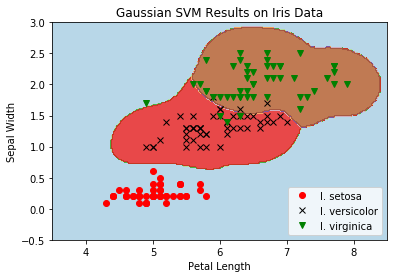
Here, we implement a 1-vs-all voting method for a multiclass SVM. We attempt to separate the three Iris flower classes with TensorFlow.

Multiclass SVM

This function wll illustrate how to implement the gaussian kernel with multiple classes on the iris dataset.

Gaussian Kernel:

X : (Sepal Length, Petal Width)

Y: (I. setosa, I. virginica, I. versicolor) (3 classes)

Basic idea: introduce an extra dimension to do one vs all classification.

The prediction of a point will be the category with the largest margin or distance to boundary.

We start by loading the necessary libraries.

1
2
3
4
5
6
import matplotlib.pyplot as plt
import numpy as np
import tensorflow as tf
from sklearn import datasets
from tensorflow.python.framework import ops
ops.reset_default_graph()

Start a computational graph session.

1
sess = tf.Session()

Now we load the iris data.

1
2
3
4
5
6
7
8
9
10
11
12
13
14
# Load the data
# iris.data = [(Sepal Length, Sepal Width, Petal Length, Petal Width)]
iris = datasets.load_iris()
x_vals = np.array([[x[0], x[3]] for x in iris.data])
y_vals1 = np.array([1 if y==0 else -1 for y in iris.target])
y_vals2 = np.array([1 if y==1 else -1 for y in iris.target])
y_vals3 = np.array([1 if y==2 else -1 for y in iris.target])
y_vals = np.array([y_vals1, y_vals2, y_vals3])
class1_x = [x[0] for i,x in enumerate(x_vals) if iris.target[i]==0]
class1_y = [x[1] for i,x in enumerate(x_vals) if iris.target[i]==0]
class2_x = [x[0] for i,x in enumerate(x_vals) if iris.target[i]==1]
class2_y = [x[1] for i,x in enumerate(x_vals) if iris.target[i]==1]
class3_x = [x[0] for i,x in enumerate(x_vals) if iris.target[i]==2]
class3_y = [x[1] for i,x in enumerate(x_vals) if iris.target[i]==2]

Declare the batch size

1
batch_size = 50

Initialize placeholders and create the variables for multiclass SVM

1
2
3
4
5
6
7
# Initialize placeholders
x_data = tf.placeholder(shape=[None, 2], dtype=tf.float32)
y_target = tf.placeholder(shape=[3, None], dtype=tf.float32)
prediction_grid = tf.placeholder(shape=[None, 2], dtype=tf.float32)

# Create variables for svm
b = tf.Variable(tf.random_normal(shape=[3,batch_size]))

Create the Gaussian Kernel

1
2
3
4
5
6
# Gaussian (RBF) kernel
gamma = tf.constant(-10.0)
dist = tf.reduce_sum(tf.square(x_data), 1)
dist = tf.reshape(dist, [-1,1])
sq_dists = tf.multiply(2., tf.matmul(x_data, tf.transpose(x_data)))
my_kernel = tf.exp(tf.multiply(gamma, tf.abs(sq_dists)))

Declare a function that will do reshaping and batch matrix multiplication

1
2
3
4
5
# Declare function to do reshape/batch multiplication
def reshape_matmul(mat, _size):
v1 = tf.expand_dims(mat, 1)
v2 = tf.reshape(v1, [3, _size, 1])
return(tf.matmul(v2, v1))

Now we can compute the SVM model

1
2
3
4
5
6
7
# Compute SVM Model
first_term = tf.reduce_sum(b)
b_vec_cross = tf.matmul(tf.transpose(b), b)
y_target_cross = reshape_matmul(y_target, batch_size)

second_term = tf.reduce_sum(tf.multiply(my_kernel, tf.multiply(b_vec_cross, y_target_cross)),[1,2])
loss = tf.reduce_sum(tf.negative(tf.subtract(first_term, second_term)))

Create the same RBF kernel for a set of prediction points (used on a grid of points at the end).

1
2
3
4
5
6
7
8
9
# Gaussian (RBF) prediction kernel
rA = tf.reshape(tf.reduce_sum(tf.square(x_data), 1),[-1,1])
rB = tf.reshape(tf.reduce_sum(tf.square(prediction_grid), 1),[-1,1])
pred_sq_dist = tf.add(tf.subtract(rA, tf.multiply(2., tf.matmul(x_data, tf.transpose(prediction_grid)))), tf.transpose(rB))
pred_kernel = tf.exp(tf.multiply(gamma, tf.abs(pred_sq_dist)))

prediction_output = tf.matmul(tf.multiply(y_target,b), pred_kernel)
prediction = tf.argmax(prediction_output-tf.expand_dims(tf.reduce_mean(prediction_output,1), 1), 0)
accuracy = tf.reduce_mean(tf.cast(tf.equal(prediction, tf.argmax(y_target,0)), tf.float32))

Create the optimization and variable initializer operations.

1
2
3
4
5
6
7
# Declare optimizer
my_opt = tf.train.GradientDescentOptimizer(0.01)
train_step = my_opt.minimize(loss)

# Initialize variables
init = tf.global_variables_initializer()
sess.run(init)

We now start the training loop for the multiclass SVM

1
2
3
4
5
6
7
8
9
10
11
12
13
14
15
16
17
18
19
20
# Training loop
loss_vec = []
batch_accuracy = []
for i in range(100):
rand_index = np.random.choice(len(x_vals), size=batch_size)
rand_x = x_vals[rand_index]
rand_y = y_vals[:,rand_index]
sess.run(train_step, feed_dict={x_data: rand_x, y_target: rand_y})

temp_loss = sess.run(loss, feed_dict={x_data: rand_x, y_target: rand_y})
loss_vec.append(temp_loss)

acc_temp = sess.run(accuracy, feed_dict={x_data: rand_x,
y_target: rand_y,
prediction_grid:rand_x})
batch_accuracy.append(acc_temp)

if (i+1)%25==0:
print('Step #' + str(i+1))
print('Loss = ' + str(temp_loss))
Step #25
Loss = -295.13718
Step #50
Loss = -632.6369
Step #75
Loss = -970.1367
Step #100
Loss = -1307.6366

For a pretty picture, to see the results, we create a fine grid of points to label/color for each class.

1
2
3
4
5
6
7
8
9
10
# Create a mesh to plot points in
x_min, x_max = x_vals[:, 0].min() - 1, x_vals[:, 0].max() + 1
y_min, y_max = x_vals[:, 1].min() - 1, x_vals[:, 1].max() + 1
xx, yy = np.meshgrid(np.arange(x_min, x_max, 0.02),
np.arange(y_min, y_max, 0.02))
grid_points = np.c_[xx.ravel(), yy.ravel()]
grid_predictions = sess.run(prediction, feed_dict={x_data: rand_x,
y_target: rand_y,
prediction_grid: grid_points})
grid_predictions = grid_predictions.reshape(xx.shape)

Plot the results

1
2
3
4
5
6
7
8
9
10
11
12
13
14
15
16
17
18
19
20
21
22
23
24
25
26
27
# Plot points and grid
plt.contourf(xx, yy, grid_predictions, cmap=plt.cm.Paired, alpha=0.8)
plt.plot(class1_x, class1_y, 'ro', label='I. setosa')
plt.plot(class2_x, class2_y, 'kx', label='I. versicolor')
plt.plot(class3_x, class3_y, 'gv', label='I. virginica')
plt.title('Gaussian SVM Results on Iris Data')
plt.xlabel('Petal Length')
plt.ylabel('Sepal Width')
plt.legend(loc='lower right')
plt.ylim([-0.5, 3.0])
plt.xlim([3.5, 8.5])
plt.show()

# Plot batch accuracy
plt.plot(batch_accuracy, 'k-', label='Accuracy')
plt.title('Batch Accuracy')
plt.xlabel('Generation')
plt.ylabel('Accuracy')
plt.legend(loc='lower right')
plt.show()

# Plot loss over time
plt.plot(loss_vec, 'k-')
plt.title('Loss per Generation')
plt.xlabel('Generation')
plt.ylabel('Loss')
plt.show()

png

png

png

本站所有文章和源码均免费开放,如您喜欢,可以请我喝杯咖啡