Nearest Neighbor methods are a very popular ML algorithm. We show how to implement k-Nearest Neighbors, weighted k-Nearest Neighbors, and k-Nearest Neighbors with mixed distance functions. In this chapter we also show how to use the Levenshtein distance (edit distance) in TensorFlow, and use it to calculate the distance between strings. We end this chapter with showing how to use k-Nearest Neighbors for categorical prediction with the MNIST handwritten digit recognition.
Nearest neighbor methods are based on a distance-based conceptual idea. We consider our training set as the model and make predictions on new points based on how close they are to points in the training set. A naïve way is to make the prediction as the closest training data point class. But since most datasets contain a degree of noise, a more common method would be to take a weighted average of a set of k nearest neighbors. This method is called k-nearest neighbors (k-NN).
Given a training dataset (x1, x2, …, xn), with corresponding targets (y1, y2, …, yn), we can make a prediction on a point, z, by looking at a set of nearest neighbors. The actual method of prediction depends on whether or not we are doing regression (continuous y) or classification (discrete y).
For discrete classification targets, the prediction may be given by a maximum voting scheme weighted by the distance to the prediction point:
prediction(z) = max ( weighted sum of distances of points in each class )
see jupyter notebook for the formula
Here, our prediction is the maximum weighted value over all classes (j), where the weighted distance from the prediction point is usually given by the L1 or L2 distance functions.
Continuous targets are very similar, but we usually just compute a weighted average of the target variable (y) by distance.
There are many different specifications of distance metrics that we can choose. In this chapter, we will explore the L1 and L2 metrics as well as edit and textual distances.
We also have to choose how to weight the distances. A straight forward way to weight the distances is by the distance itself. Points that are further away from our prediction should have less impact than nearer points. The most common way to weight is by the normalized inverse of the distance. We will implement this method in the next recipe.
Note that k-NN is an aggregating method. For regression, we are performing a weighted average of neighbors. Because of this, predictions will be less extreme and less varied than the actual targets. The magnitude of this effect will be determined by k, the number of neighbors in the algorithm.
This function illustrates how to use k-nearest neighbors in tensorflow
We will use the 1970s Boston housing dataset which is available through the UCI ML data repository.
Data:
—————x-values—————-
CRIM : per capita crime rate by town
ZN : prop. of res. land zones
INDUS : prop. of non-retail business acres
CHAS : Charles river dummy variable
NOX : nitrix oxides concentration / 10 M
RM : Avg. # of rooms per building
AGE : prop. of buildings built prior to 1940
DIS : Weighted distances to employment centers
RAD : Index of radian highway access
TAX : Full tax rate value per $10k
PTRATIO: Pupil/Teacher ratio by town
B : 1000*(Bk-0.63)^2, Bk=prop. of blacks
LSTAT : % lower status of pop
——————y-value—————-
MEDV : Median Value of homes in $1,000’s
1
2
3
4
5
6
7
# import required libraries
import matplotlib.pyplot as plt
import numpy as np
import tensorflow as tf
import requests
from tensorflow.python.framework import ops
ops.reset_default_graph()
Create graph
1
sess = tf.Session()
Load the data
1
2
3
4
5
6
7
8
9
10
11
12
housing_url = 'https://archive.ics.uci.edu/ml/machine-learning-databases/housing/housing.data' housing_header = ['CRIM', 'ZN', 'INDUS', 'CHAS', 'NOX', 'RM', 'AGE', 'DIS', 'RAD', 'TAX', 'PTRATIO', 'B', 'LSTAT', 'MEDV'] cols_used = ['CRIM', 'INDUS', 'NOX', 'RM', 'AGE', 'DIS', 'TAX', 'PTRATIO', 'B', 'LSTAT'] num_features = len(cols_used) housing_file = requests.get(housing_url) housing_data = [[float(x) for x in y.split(' ') if len(x)>=1] for y in housing_file.text.split('\n') if len(y)>=1]
y_vals = np.transpose([np.array([y[13] for y in housing_data])]) x_vals = np.array([[x for i,x in enumerate(y) if housing_header[i] in cols_used] for y in housing_data])
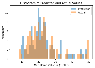
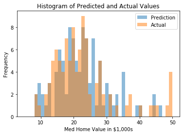
%matplotlib inline # Plot prediction and actual distribution bins = np.linspace(5, 50, 45)
plt.hist(predictions, bins, alpha=0.5, label='Prediction') plt.hist(y_batch, bins, alpha=0.5, label='Actual') plt.title('Histogram of Predicted and Actual Values') plt.xlabel('Med Home Value in $1,000s') plt.ylabel('Frequency') plt.legend(loc='upper right') plt.show()
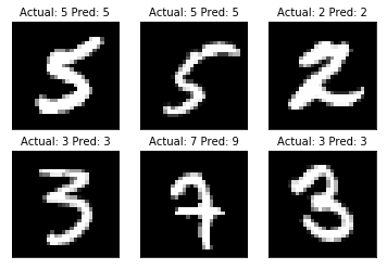
This script will load the MNIST data, and split it into test/train and perform prediction with nearest neighbors.
For each test integer, we will return the closest image/integer.
Integer images are represented as 28x28 matrices of floating point numbers.
1 2 3 4 5 6 7 8
import random import numpy as np import tensorflow as tf import matplotlib.pyplot as plt from PIL import Image from tensorflow.examples.tutorials.mnist import input_data from tensorflow.python.framework import ops ops.reset_default_graph()
num_h_words = len(hypothesis_words) h_indices = [[xi, 0, yi] for xi,x in enumerate(hypothesis_words) for yi,y in enumerate(x)] h_chars = list(''.join(hypothesis_words))
truth_word_vec = truth_word*num_h_words t_indices = [[xi, 0, yi] for xi,x in enumerate(truth_word_vec) for yi,y in enumerate(x)] t_chars = list(''.join(truth_word_vec))
t3 = tf.SparseTensor(t_indices, t_chars, [num_h_words,1,1])
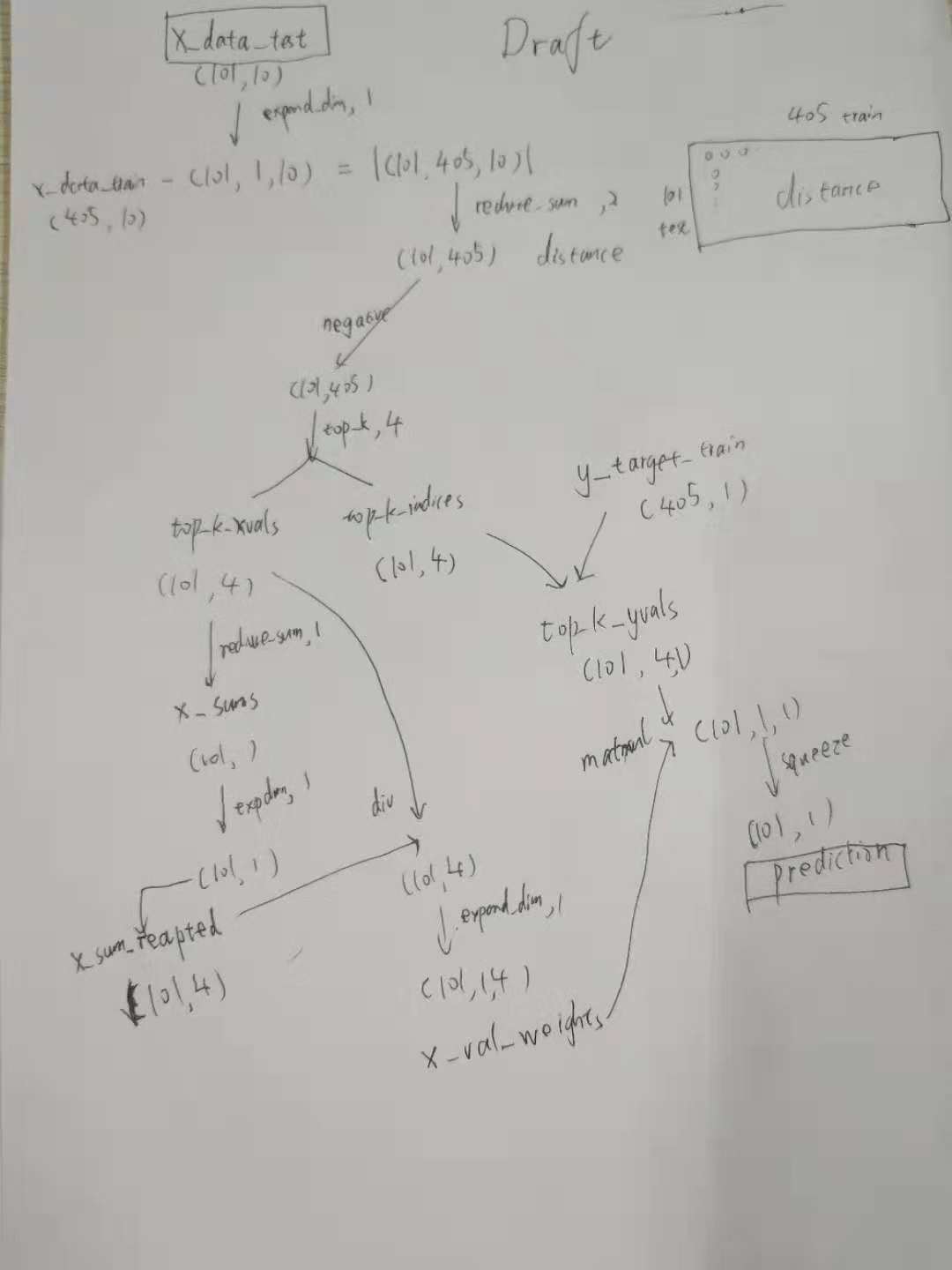
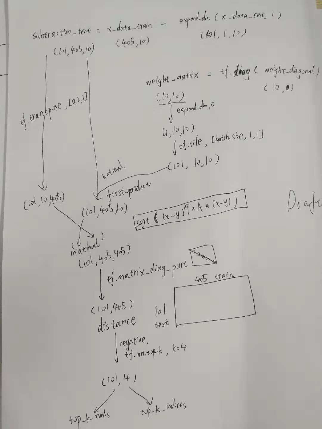
This function shows how to use different distance metrics on different features for kNN.
Data:
—————x-values—————-
CRIM : per capita crime rate by town
ZN : prop. of res. land zones
INDUS : prop. of non-retail business acres
CHAS : Charles river dummy variable
NOX : nitrix oxides concentration / 10 M
RM : Avg. # of rooms per building
AGE : prop. of buildings built prior to 1940
DIS : Weighted distances to employment centers
RAD : Index of radian highway access
TAX : Full tax rate value per $10k
PTRATIO: Pupil/Teacher ratio by town
B : 1000*(Bk-0.63)^2, Bk=prop. of blacks
LSTAT : % lower status of pop
——————y-value—————-
MEDV : Median Value of homes in $1,000’s
1 2 3 4 5 6
import matplotlib.pyplot as plt import numpy as np import tensorflow as tf import requests from tensorflow.python.framework import ops ops.reset_default_graph()
housing_url = 'https://archive.ics.uci.edu/ml/machine-learning-databases/housing/housing.data' housing_header = ['CRIM', 'ZN', 'INDUS', 'CHAS', 'NOX', 'RM', 'AGE', 'DIS', 'RAD', 'TAX', 'PTRATIO', 'B', 'LSTAT', 'MEDV'] cols_used = ['CRIM', 'INDUS', 'NOX', 'RM', 'AGE', 'DIS', 'TAX', 'PTRATIO', 'B', 'LSTAT'] num_features = len(cols_used) housing_file = requests.get(housing_url) housing_data = [[float(x) for x in y.split(' ') if len(x)>=1] for y in housing_file.text.split('\n') if len(y)>=1]
y_vals = np.transpose([np.array([y[13] for y in housing_data])]) x_vals = np.array([[x for i,x in enumerate(y) if housing_header[i] in cols_used] for y in housing_data])
%matplotlib inline
# Plot prediction and actual distribution
bins = np.linspace(5, 50, 45)

plt.hist(predictions, bins, alpha=0.5, label='Prediction')
plt.hist(y_batch, bins, alpha=0.5, label='Actual')
plt.title('Histogram of Predicted and Actual Values')
plt.xlabel('Med Home Value in $1,000s')
plt.ylabel('Frequency')
plt.legend(loc='upper right')
plt.show()
# n = Size of created data sets n = 10 street_names = ['abbey', 'baker', 'canal', 'donner', 'elm'] street_types = ['rd', 'st', 'ln', 'pass', 'ave']
random.seed(31) #make results reproducible rand_zips = [random.randint(65000,65999) for i in range(5)]
# Function to randomly create one typo in a string w/ a probability defcreate_typo(s, prob=0.75): if random.uniform(0,1) < prob: rand_ind = random.choice(range(len(s))) s_list = list(s) s_list[rand_ind]=random.choice(string.ascii_lowercase) s = ''.join(s_list) return(s)
# Generate the reference dataset numbers = [random.randint(1, 9999) for i in range(n)] streets = [random.choice(street_names) for i in range(n)] street_suffs = [random.choice(street_types) for i in range(n)] zips = [random.choice(rand_zips) for i in range(n)] full_streets = [str(x) + ' ' + y + ' ' + z for x,y,z in zip(numbers, streets, street_suffs)] reference_data = [list(x) for x in zip(full_streets,zips)]
# Generate test dataset with some typos typo_streets = [create_typo(x) for x in streets] typo_full_streets = [str(x) + ' ' + y + ' ' + z for x,y,z in zip(numbers, typo_streets, street_suffs)] test_data = [list(x) for x in zip(typo_full_streets,zips)]
# Predict: Get max similarity entry top_match_index = tf.argmax(weighted_sim, 1)
# Function to Create a character-sparse tensor from strings defsparse_from_word_vec(word_vec): num_words = len(word_vec) indices = [[xi, 0, yi] for xi,x in enumerate(word_vec) for yi,y in enumerate(x)] chars = list(''.join(word_vec)) return(tf.SparseTensorValue(indices, chars, [num_words,1,1]))