0%

神经网络 Neural Networks

神经网络

Neural Network
(人工)神经网络是一种起源于 20 世纪 50 年代的监督式机器学习模型,那时候研究者构想了「感知器(perceptron)」的想法。这一领域的研究者通常被称为「联结主义者(Connectionist)」,因为这种模型模拟了人脑的功能。神经网络模型通常是通过反向传播算法应用梯度下降训练的。目前神经网络有两大主要类型,它们是前馈神经网络(主要是卷积神经网络-CNN)和循环神经网络(RNN),其中 RNN 又包含长短期记忆(LSTM)、门控循环单元(GRU)等子类。深度学习(deep learning)是一种主要应用于神经网络技术以帮助其取得更好结果的技术。尽管神经网络主要用于监督学习,但也有一些为无监督学习设计的变体,如自动编码器(AutoEncoder)和生成对抗网络(GAN)。

Introduction to Neural Networks

There are more resources for learning about neural networks that are more in depth and detailed. Here are some following resources:

Implementing Gates

This function shows how to implement various gates in TensorFlow.

One gate will be one operation with a variable and a placeholder. We will ask TensorFlow
to change the variable based on our loss function

1
2
3
import tensorflow as tf
from tensorflow.python.framework import ops
ops.reset_default_graph()

Gate 1

Create a multiplication gate: $f(x) = a * x$

1
2
3
4
5
a --
|
|---- (multiply) --> output
|
x --

1
2
3
4
5
6
7
8
9
10
11
12
13
14
15
16
17
18
19
20
21
22
23
24
25
26
27
28
# Start Graph Session
sess = tf.Session()

a = tf.Variable(tf.constant(4.))
x_val = 5.
x_data = tf.placeholder(dtype=tf.float32)

multiplication = tf.multiply(a, x_data)

# Declare the loss function as the difference between
# the output and a target value, 50.
loss = tf.square(tf.subtract(multiplication, 50.))

# Initialize variables
init = tf.global_variables_initializer()
sess.run(init)

# Declare optimizer
my_opt = tf.train.GradientDescentOptimizer(0.01)
train_step = my_opt.minimize(loss)

# Run loop across gate
print('Optimizing a Multiplication Gate Output to 50.')
for i in range(10):
sess.run(train_step, feed_dict={x_data: x_val})
a_val = sess.run(a)
mult_output = sess.run(multiplication, feed_dict={x_data: x_val})
print(str(a_val) + ' * ' + str(x_val) + ' = ' + str(mult_output))
Optimizing a Multiplication Gate Output to 50.
7.0 * 5.0 = 35.0
8.5 * 5.0 = 42.5
9.25 * 5.0 = 46.25
9.625 * 5.0 = 48.125
9.8125 * 5.0 = 49.0625
9.90625 * 5.0 = 49.53125
9.953125 * 5.0 = 49.765625
9.9765625 * 5.0 = 49.882812
9.988281 * 5.0 = 49.941406
9.994141 * 5.0 = 49.970703

Gate 2

Create a nested gate: $f(x) = a * x + b$

1
2
3
4
5
6
7
a --
|
|-- (multiply)--
| |
x -- |-- (add) --> output
|
b --
1
2
3
4
5
6
7
8
9
10
11
12
13
14
15
16
17
18
19
20
21
22
23
24
25
26
27
28
29
30
# Start a New Graph Session
ops.reset_default_graph()
sess = tf.Session()

a = tf.Variable(tf.constant(1.))
b = tf.Variable(tf.constant(1.))
x_val = 5.
x_data = tf.placeholder(dtype=tf.float32)

two_gate = tf.add(tf.multiply(a, x_data), b)

# Declare the loss function as the difference between
# the output and a target value, 50.
loss = tf.square(tf.subtract(two_gate, 50.))

# Initialize variables
init = tf.global_variables_initializer()
sess.run(init)

# Declare optimizer
my_opt = tf.train.GradientDescentOptimizer(0.01)
train_step = my_opt.minimize(loss)

# Run loop across gate
print('\nOptimizing Two Gate Output to 50.')
for i in range(10):
sess.run(train_step, feed_dict={x_data: x_val})
a_val, b_val = (sess.run(a), sess.run(b))
two_gate_output = sess.run(two_gate, feed_dict={x_data: x_val})
print(str(a_val) + ' * ' + str(x_val) + ' + ' + str(b_val) + ' = ' + str(two_gate_output))
Optimizing Two Gate Output to 50.
5.4 * 5.0 + 1.88 = 28.88
7.512 * 5.0 + 2.3024 = 39.8624
8.52576 * 5.0 + 2.5051522 = 45.133953
9.012364 * 5.0 + 2.6024733 = 47.664295
9.2459345 * 5.0 + 2.6491873 = 48.87886
9.358048 * 5.0 + 2.67161 = 49.461853
9.411863 * 5.0 + 2.682373 = 49.74169
9.437695 * 5.0 + 2.687539 = 49.87601
9.450093 * 5.0 + 2.690019 = 49.940483
9.456045 * 5.0 + 2.6912093 = 49.971436

Combining Gates and Activation Functions

This function shows how to implement various gates with activation functions in TensorFlow.

This function is an extension of the prior gates, but with various activation functions.

1
2
3
4
5
import tensorflow as tf
import numpy as np
import matplotlib.pyplot as plt
from tensorflow.python.framework import ops
ops.reset_default_graph()
1
2
3
4
5
6
7
8
9
10
11
12
13
14
15
16
17
# Start Graph Session
sess = tf.Session()
tf.set_random_seed(5)
np.random.seed(42)

batch_size = 50

a1 = tf.Variable(tf.random_normal(shape=[1,1]))
b1 = tf.Variable(tf.random_uniform(shape=[1,1]))
a2 = tf.Variable(tf.random_normal(shape=[1,1]))
b2 = tf.Variable(tf.random_uniform(shape=[1,1]))
x = np.random.normal(2, 0.1, 500)
x_data = tf.placeholder(shape=[None, 1], dtype=tf.float32)

sigmoid_activation = tf.sigmoid(tf.add(tf.matmul(x_data, a1), b1))

relu_activation = tf.nn.relu(tf.add(tf.matmul(x_data, a2), b2))
1
2
3
4
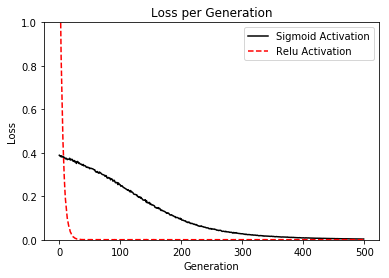
# Declare the loss function as the difference between
# the output and a target value, 0.75.
loss1 = tf.reduce_mean(tf.square(tf.subtract(sigmoid_activation, 0.75)))
loss2 = tf.reduce_mean(tf.square(tf.subtract(relu_activation, 0.75)))
1
2
3
# Initialize variables
init = tf.global_variables_initializer()
sess.run(init)
1
2
3
4
# Declare optimizer
my_opt = tf.train.GradientDescentOptimizer(0.01)
train_step_sigmoid = my_opt.minimize(loss1)
train_step_relu = my_opt.minimize(loss2)
1
2
3
4
5
6
7
8
9
10
11
12
13
14
15
16
17
18
# Run loop across gate
print('\nOptimizing Sigmoid AND Relu Output to 0.75')
loss_vec_sigmoid = []
loss_vec_relu = []
for i in range(500):
rand_indices = np.random.choice(len(x), size=batch_size)
x_vals = np.transpose([x[rand_indices]])
sess.run(train_step_sigmoid, feed_dict={x_data: x_vals})
sess.run(train_step_relu, feed_dict={x_data: x_vals})

loss_vec_sigmoid.append(sess.run(loss1, feed_dict={x_data: x_vals}))
loss_vec_relu.append(sess.run(loss2, feed_dict={x_data: x_vals}))

sigmoid_output = np.mean(sess.run(sigmoid_activation, feed_dict={x_data: x_vals}))
relu_output = np.mean(sess.run(relu_activation, feed_dict={x_data: x_vals}))

if i%50==0:
print('sigmoid = ' + str(np.mean(sigmoid_output)) + ' relu = ' + str(np.mean(relu_output)))
Optimizing Sigmoid AND Relu Output to 0.75
sigmoid = 0.12655208 relu = 2.0227606
sigmoid = 0.17863758 relu = 0.7530296
sigmoid = 0.24769811 relu = 0.7492897
sigmoid = 0.3446748 relu = 0.7499546
sigmoid = 0.4400661 relu = 0.7539999
sigmoid = 0.5236898 relu = 0.754772
sigmoid = 0.58373857 relu = 0.7508698
sigmoid = 0.62733483 relu = 0.7470234
sigmoid = 0.6549499 relu = 0.75180537
sigmoid = 0.67452586 relu = 0.75470716
1
2
3
4
5
6
7
8
9
# Plot the loss
plt.plot(loss_vec_sigmoid, 'k-', label='Sigmoid Activation')
plt.plot(loss_vec_relu, 'r--', label='Relu Activation')
plt.ylim([0, 1.0])
plt.title('Loss per Generation')
plt.xlabel('Generation')
plt.ylabel('Loss')
plt.legend(loc='upper right')
plt.show()

png


Implementing a one-layer Neural Network

Model

The model will have one hidden layer. If the hidden layer has 10 nodes, then the model will look like the following:

One Hidden Layer Network

We will use the ReLU activation functions.

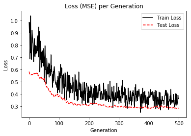
For the loss function, we will use the average MSE across the batch.
We will illustrate how to create a one hidden layer NN

We will use the iris data for this exercise

We will build a one-hidden layer neural network to predict the fourth attribute, Petal Width from the other three (Sepal length, Sepal width, Petal length).

1
2
3
4
5
import matplotlib.pyplot as plt
import numpy as np
import tensorflow as tf
from sklearn import datasets
from tensorflow.python.framework import ops
1
ops.reset_default_graph()
1
2
3
iris = datasets.load_iris()
x_vals = np.array([x[0:3] for x in iris.data])
y_vals = np.array([x[3] for x in iris.data])
1
2
# Create graph session
sess = tf.Session()
1
2
3
4
# make results reproducible
seed = 2
tf.set_random_seed(seed)
np.random.seed(seed)
1
2
3
4
5
6
7
# Split data into train/test = 80%/20%
train_indices = np.random.choice(len(x_vals), round(len(x_vals)*0.8), replace=False)
test_indices = np.array(list(set(range(len(x_vals))) - set(train_indices)))
x_vals_train = x_vals[train_indices]
x_vals_test = x_vals[test_indices]
y_vals_train = y_vals[train_indices]
y_vals_test = y_vals[test_indices]
1
2
3
4
5
6
7
8
# Normalize by column (min-max norm)
def normalize_cols(m):
col_max = m.max(axis=0)
col_min = m.min(axis=0)
return (m-col_min) / (col_max - col_min)

x_vals_train = np.nan_to_num(normalize_cols(x_vals_train))
x_vals_test = np.nan_to_num(normalize_cols(x_vals_test))
1
2
3
4
5
6
# Declare batch size
batch_size = 50

# Initialize placeholders
x_data = tf.placeholder(shape=[None, 3], dtype=tf.float32)
y_target = tf.placeholder(shape=[None, 1], dtype=tf.float32)
1
2
3
4
5
6
7
8
9
10
11
12
13
14
15
16
17
18
# Create variables for both NN layers
hidden_layer_nodes = 10
A1 = tf.Variable(tf.random_normal(shape=[3,hidden_layer_nodes])) # inputs -> hidden nodes
b1 = tf.Variable(tf.random_normal(shape=[hidden_layer_nodes])) # one biases for each hidden node
A2 = tf.Variable(tf.random_normal(shape=[hidden_layer_nodes,1])) # hidden inputs -> 1 output
b2 = tf.Variable(tf.random_normal(shape=[1])) # 1 bias for the output


# Declare model operations
hidden_output = tf.nn.relu(tf.add(tf.matmul(x_data, A1), b1))
final_output = tf.nn.relu(tf.add(tf.matmul(hidden_output, A2), b2))

# Declare loss function (MSE)
loss = tf.reduce_mean(tf.square(y_target - final_output))

# Declare optimizer
my_opt = tf.train.GradientDescentOptimizer(0.005)
train_step = my_opt.minimize(loss)
1
2
3
4
5
6
7
8
9
10
11
12
13
14
15
16
17
18
19
20
# Initialize variables
init = tf.global_variables_initializer()
sess.run(init)

# Training loop
loss_vec = []
test_loss = []
for i in range(500):
rand_index = np.random.choice(len(x_vals_train), size=batch_size)
rand_x = x_vals_train[rand_index]
rand_y = np.transpose([y_vals_train[rand_index]])
sess.run(train_step, feed_dict={x_data: rand_x, y_target: rand_y})

temp_loss = sess.run(loss, feed_dict={x_data: rand_x, y_target: rand_y})
loss_vec.append(np.sqrt(temp_loss))

test_temp_loss = sess.run(loss, feed_dict={x_data: x_vals_test, y_target: np.transpose([y_vals_test])})
test_loss.append(np.sqrt(test_temp_loss))
if (i+1)%50==0:
print('Generation: ' + str(i+1) + '. Loss = ' + str(temp_loss))
Generation: 50. Loss = 0.5279015
Generation: 100. Loss = 0.22871476
Generation: 150. Loss = 0.17977345
Generation: 200. Loss = 0.10849865
Generation: 250. Loss = 0.24002916
Generation: 300. Loss = 0.15323998
Generation: 350. Loss = 0.1659011
Generation: 400. Loss = 0.09752482
Generation: 450. Loss = 0.121614255
Generation: 500. Loss = 0.1300937
1
2
3
4
5
6
7
8
9
%matplotlib inline
# Plot loss (MSE) over time
plt.plot(loss_vec, 'k-', label='Train Loss')
plt.plot(test_loss, 'r--', label='Test Loss')
plt.title('Loss (MSE) per Generation')
plt.legend(loc='upper right')
plt.xlabel('Generation')
plt.ylabel('Loss')
plt.show()

png


Implementing Different Layers

We will illustrate how to use different types of layers in TensorFlow

The layers of interest are:

  1. Convolutional Layer
  2. Activation Layer
  3. Max-Pool Layer
  4. Fully Connected Layer

We will generate two different data sets for this script, a 1-D data set (row of data) and a 2-D data set (similar to picture)

1
2
3
4
5
6
7
8
import tensorflow as tf
import matplotlib.pyplot as plt
import csv
import os
import random
import numpy as np
import random
from tensorflow.python.framework import ops
1
2
3
#---------------------------------------------------|
#-------------------1D-data-------------------------|
#---------------------------------------------------|
1
2
3
4
5
6
7
8
9
10
11
12
13
14
15
16
17
18
19
20
21
22
23
24
25
26
27
28
29
30
31
32
33
34
35
36
37
38
39
40
41
42
43
44
45
46
47
48
49
50
51
52
53
54
55
56
57
58
59
60
61
62
63
64
65
66
67
68
69
70
71
72
73
74
75
76
77
78
79
80
81
82
83
84
85
86
87
88
# Create graph session
ops.reset_default_graph()
sess = tf.Session()

# parameters for the run
data_size = 25
conv_size = 5
maxpool_size = 5
stride_size = 1

# ensure reproducibility
seed=13
np.random.seed(seed)
tf.set_random_seed(seed)

# Generate 1D data
data_1d = np.random.normal(size=data_size)

# Placeholder
x_input_1d = tf.placeholder(dtype=tf.float32, shape=[data_size])

#--------Convolution--------
# both [batch#, width, height, channels] and [batch#, height, width, channels] are correct.Nut (input, filter, strides, padding) dimensional relations should keep correspondence.
def conv_layer_1d(input_1d, my_filter,stride):
# TensorFlow's 'conv2d()' function only works with 4D arrays:
# [batch#, width, height, channels], we have 1 batch, and
# width = 1, but height = the length of the input, and 1 channel.
# So next we create the 4D array by inserting dimension 1's.
input_2d = tf.expand_dims(input_1d, 0)
input_3d = tf.expand_dims(input_2d, 0)
input_4d = tf.expand_dims(input_3d, 3)
# Perform convolution with stride = 1, if we wanted to increase the stride,
# to say '2', then strides=[1,1,2,1]
convolution_output = tf.nn.conv2d(input_4d, filter=my_filter, strides=[1,1,stride,1], padding="VALID")
# Get rid of extra dimensions
conv_output_1d = tf.squeeze(convolution_output)
return(conv_output_1d)

# Create filter for convolution.
my_filter = tf.Variable(tf.random_normal(shape=[1,conv_size,1,1]))
# Create convolution layer
my_convolution_output = conv_layer_1d(x_input_1d, my_filter,stride=stride_size)

#--------Activation--------
def activation(input_1d):
return(tf.nn.relu(input_1d))

# Create activation layer
my_activation_output = activation(my_convolution_output)

#--------Max Pool--------
def max_pool(input_1d, width,stride):
# Just like 'conv2d()' above, max_pool() works with 4D arrays.
# [batch_size=1, width=1, height=num_input, channels=1]
input_2d = tf.expand_dims(input_1d, 0)
input_3d = tf.expand_dims(input_2d, 0)
input_4d = tf.expand_dims(input_3d, 3)
# Perform the max pooling with strides = [1,1,1,1]
# If we wanted to increase the stride on our data dimension, say by
# a factor of '2', we put strides = [1, 1, 2, 1]
# We will also need to specify the width of the max-window ('width')
pool_output = tf.nn.max_pool(input_4d, ksize=[1, 1, width, 1],
strides=[1, 1, stride, 1],
padding='VALID')
# Get rid of extra dimensions
pool_output_1d = tf.squeeze(pool_output)
return(pool_output_1d)

my_maxpool_output = max_pool(my_activation_output, width=maxpool_size,stride=stride_size)

#--------Fully Connected--------
def fully_connected(input_layer, num_outputs):
# First we find the needed shape of the multiplication weight matrix:
# The dimension will be (length of input) by (num_outputs)
weight_shape = tf.squeeze(tf.stack([tf.shape(input_layer),[num_outputs]]))
# Initialize such weight
weight = tf.random_normal(weight_shape, stddev=0.1)
# Initialize the bias
bias = tf.random_normal(shape=[num_outputs])
# Make the 1D input array into a 2D array for matrix multiplication
input_layer_2d = tf.expand_dims(input_layer, 0)
# Perform the matrix multiplication and add the bias
full_output = tf.add(tf.matmul(input_layer_2d, weight), bias)
# Get rid of extra dimensions
full_output_1d = tf.squeeze(full_output)
return(full_output_1d)

my_full_output = fully_connected(my_maxpool_output, 5)
1
2
3
4
5
6
7
8
9
10
11
12
13
14
15
16
17
18
19
20
21
22
23
24
25
26
27
28
29
30
31
# Run graph
# Initialize Variables
init = tf.global_variables_initializer()
sess.run(init)

feed_dict = {x_input_1d: data_1d}

print('>>>> 1D Data <<<<')

# Convolution Output
print('Input = array of length %d' % (x_input_1d.shape.as_list()[0]))
print('Convolution w/ filter, length = %d, stride size = %d, results in an array of length %d:' %
(conv_size,stride_size,my_convolution_output.shape.as_list()[0]))
print(sess.run(my_convolution_output, feed_dict=feed_dict))

# Activation Output
print('\nInput = above array of length %d' % (my_convolution_output.shape.as_list()[0]))
print('ReLU element wise returns an array of length %d:' % (my_activation_output.shape.as_list()[0]))
print(sess.run(my_activation_output, feed_dict=feed_dict))

# Max Pool Output
print('\nInput = above array of length %d' % (my_activation_output.shape.as_list()[0]))
print('MaxPool, window length = %d, stride size = %d, results in the array of length %d' %
(maxpool_size,stride_size,my_maxpool_output.shape.as_list()[0]))
print(sess.run(my_maxpool_output, feed_dict=feed_dict))

# Fully Connected Output
print('\nInput = above array of length %d' % (my_maxpool_output.shape.as_list()[0]))
print('Fully connected layer on all 4 rows with %d outputs:' %
(my_full_output.shape.as_list()[0]))
print(sess.run(my_full_output, feed_dict=feed_dict))
>>>> 1D Data <<<<
Input = array of length 25
Convolution w/ filter, length = 5, stride size = 1, results in an array of length 21:
[-2.63576341 -1.11550486 -0.95571411 -1.69670296 -0.35699379  0.62266493
  4.43316031  2.01364899  1.33044648 -2.30629659 -0.82916248 -2.63594174
  0.76669347 -2.46465087 -2.2855041   1.49780679  1.6960566   1.48557389
 -2.79799461  1.18149185  1.42146575]

Input = above array of length 21
ReLU element wise returns an array of length 21:
[ 0.          0.          0.          0.          0.          0.62266493
  4.43316031  2.01364899  1.33044648  0.          0.          0.
  0.76669347  0.          0.          1.49780679  1.6960566   1.48557389
  0.          1.18149185  1.42146575]

Input = above array of length 21
MaxPool, window length = 5, stride size = 1, results in the array of length 17
[ 0.          0.62266493  4.43316031  4.43316031  4.43316031  4.43316031
  4.43316031  2.01364899  1.33044648  0.76669347  0.76669347  1.49780679
  1.6960566   1.6960566   1.6960566   1.6960566   1.6960566 ]

Input = above array of length 17
Fully connected layer on all 4 rows with 5 outputs:
[ 1.71536076 -0.72340977 -1.22485089 -2.5412786  -0.16338301]
1
2
3
#---------------------------------------------------|
#-------------------2D-data-------------------------|
#---------------------------------------------------|
1
2
3
4
5
6
7
8
9
10
11
12
13
14
15
16
17
18
19
20
21
22
23
24
25
26
27
28
29
30
31
32
33
34
35
36
37
38
39
40
41
42
43
44
45
46
47
48
49
50
51
52
53
54
55
56
57
58
59
60
61
62
63
64
65
66
67
68
69
70
71
72
73
74
75
76
77
78
79
80
81
82
83
84
85
86
87
88
89
90
91
92
93
94
95
# Reset Graph
ops.reset_default_graph()
sess = tf.Session()

# parameters for the run
row_size = 10
col_size = 10
conv_size = 2
conv_stride_size = 2
maxpool_size = 2
maxpool_stride_size = 1


# ensure reproducibility
seed=13
np.random.seed(seed)
tf.set_random_seed(seed)

#Generate 2D data
data_size = [row_size,col_size]
data_2d = np.random.normal(size=data_size)

#--------Placeholder--------
x_input_2d = tf.placeholder(dtype=tf.float32, shape=data_size)

# Convolution
def conv_layer_2d(input_2d, my_filter,stride_size):
# TensorFlow's 'conv2d()' function only works with 4D arrays:
# [batch#, width, height, channels], we have 1 batch, and
# 1 channel, but we do have width AND height this time.
# So next we create the 4D array by inserting dimension 1's.
input_3d = tf.expand_dims(input_2d, 0)
input_4d = tf.expand_dims(input_3d, 3)
# Note the stride difference below!
convolution_output = tf.nn.conv2d(input_4d, filter=my_filter,
strides=[1,stride_size,stride_size,1], padding="VALID")
# Get rid of unnecessary dimensions
conv_output_2d = tf.squeeze(convolution_output)
return(conv_output_2d)

# Create Convolutional Filter
my_filter = tf.Variable(tf.random_normal(shape=[conv_size,conv_size,1,1]))
# Create Convolutional Layer
my_convolution_output = conv_layer_2d(x_input_2d, my_filter,stride_size=conv_stride_size)

#--------Activation--------
def activation(input_1d):
return(tf.nn.relu(input_1d))

# Create Activation Layer
my_activation_output = activation(my_convolution_output)

#--------Max Pool--------
def max_pool(input_2d, width, height,stride):
# Just like 'conv2d()' above, max_pool() works with 4D arrays.
# [batch_size=1, width=given, height=given, channels=1]
input_3d = tf.expand_dims(input_2d, 0)
input_4d = tf.expand_dims(input_3d, 3)
# Perform the max pooling with strides = [1,1,1,1]
# If we wanted to increase the stride on our data dimension, say by
# a factor of '2', we put strides = [1, 2, 2, 1]
pool_output = tf.nn.max_pool(input_4d, ksize=[1, height, width, 1],
strides=[1, stride, stride, 1],
padding='VALID')
# Get rid of unnecessary dimensions
pool_output_2d = tf.squeeze(pool_output)
return(pool_output_2d)

# Create Max-Pool Layer
my_maxpool_output = max_pool(my_activation_output,
width=maxpool_size, height=maxpool_size,stride=maxpool_stride_size)


#--------Fully Connected--------
def fully_connected(input_layer, num_outputs):
# In order to connect our whole W byH 2d array, we first flatten it out to
# a W times H 1D array.
flat_input = tf.reshape(input_layer, [-1])
# We then find out how long it is, and create an array for the shape of
# the multiplication weight = (WxH) by (num_outputs)
weight_shape = tf.squeeze(tf.stack([tf.shape(flat_input),[num_outputs]]))
# Initialize the weight
weight = tf.random_normal(weight_shape, stddev=0.1)
# Initialize the bias
bias = tf.random_normal(shape=[num_outputs])
# Now make the flat 1D array into a 2D array for multiplication
input_2d = tf.expand_dims(flat_input, 0)
# Multiply and add the bias
full_output = tf.add(tf.matmul(input_2d, weight), bias)
# Get rid of extra dimension
full_output_2d = tf.squeeze(full_output)
return(full_output_2d)

# Create Fully Connected Layer
my_full_output = fully_connected(my_maxpool_output, 5)
1
2
3
4
5
6
7
8
9
10
11
12
13
14
15
16
17
18
19
20
21
22
23
24
25
26
27
28
29
30
31
# Run graph
# Initialize Variables
init = tf.global_variables_initializer()
sess.run(init)

feed_dict = {x_input_2d: data_2d}

print('>>>> 2D Data <<<<')

# Convolution Output
print('Input = %s array' % (x_input_2d.shape.as_list()))
print('%s Convolution, stride size = [%d, %d] , results in the %s array' %
(my_filter.get_shape().as_list()[:2],conv_stride_size,conv_stride_size,my_convolution_output.shape.as_list()))
print(sess.run(my_convolution_output, feed_dict=feed_dict))

# Activation Output
print('\nInput = the above %s array' % (my_convolution_output.shape.as_list()))
print('ReLU element wise returns the %s array' % (my_activation_output.shape.as_list()))
print(sess.run(my_activation_output, feed_dict=feed_dict))

# Max Pool Output
print('\nInput = the above %s array' % (my_activation_output.shape.as_list()))
print('MaxPool, stride size = [%d, %d], results in %s array' %
(maxpool_stride_size,maxpool_stride_size,my_maxpool_output.shape.as_list()))
print(sess.run(my_maxpool_output, feed_dict=feed_dict))

# Fully Connected Output
print('\nInput = the above %s array' % (my_maxpool_output.shape.as_list()))
print('Fully connected layer on all %d rows results in %s outputs:' %
(my_maxpool_output.shape.as_list()[0],my_full_output.shape.as_list()[0]))
print(sess.run(my_full_output, feed_dict=feed_dict))
>>>> 2D Data <<<<
Input = [10, 10] array
[2, 2] Convolution, stride size = [2, 2] , results in the [5, 5] array
[[ 0.14431179  0.7278337   1.5114917  -1.2809976   1.7843919 ]
 [-2.5450306   0.76156765 -0.51650006  0.7713109   0.37542343]
 [ 0.4934591   0.01592223  0.38653135 -1.4799767   0.6952765 ]
 [-0.34617192 -2.5318975  -0.9525758  -1.4357065   0.6625736 ]
 [-1.9854026   0.34398788  2.5376048  -0.8678482  -0.3100495 ]]

Input = the above [5, 5] array
ReLU element wise returns the [5, 5] array
[[0.14431179 0.7278337  1.5114917  0.         1.7843919 ]
 [0.         0.76156765 0.         0.7713109  0.37542343]
 [0.4934591  0.01592223 0.38653135 0.         0.6952765 ]
 [0.         0.         0.         0.         0.6625736 ]
 [0.         0.34398788 2.5376048  0.         0.        ]]

Input = the above [5, 5] array
MaxPool, stride size = [1, 1], results in [4, 4] array
[[0.76156765 1.5114917  1.5114917  1.7843919 ]
 [0.76156765 0.76156765 0.7713109  0.7713109 ]
 [0.4934591  0.38653135 0.38653135 0.6952765 ]
 [0.34398788 2.5376048  2.5376048  0.6625736 ]]

Input = the above [4, 4] array
Fully connected layer on all 4 rows results in 5 outputs:
[ 0.08245847 -0.16351229 -0.55429065 -0.24322605 -0.99900764]

Using a Multiple Layer Network

We will illustrate how to use a Multiple Layer Network in TensorFlow

Low Birthrate data:

1
2
3
4
5
6
7
8
9
10
11
12
13
#Columns    Variable                                      Abbreviation
#---------------------------------------------------------------------
# Low Birth Weight (0 = Birth Weight >= 2500g, LOW
# 1 = Birth Weight < 2500g)
# Age of the Mother in Years AGE
# Weight in Pounds at the Last Menstrual Period LWT
# Race (1 = White, 2 = Black, 3 = Other) RACE
# Smoking Status During Pregnancy (1 = Yes, 0 = No) SMOKE
# History of Premature Labor (0 = None 1 = One, etc.) PTL
# History of Hypertension (1 = Yes, 0 = No) HT
# Presence of Uterine Irritability (1 = Yes, 0 = No) UI
# Birth Weight in Grams BWT
#---------------------------------------------------------------------

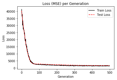
The multiple neural network layer we will create will be composed of three fully connected hidden layers, with node sizes 50, 25, and 5

1
2
3
4
5
6
7
8
9
10
import tensorflow as tf
import matplotlib.pyplot as plt
import csv
import os
import os.path
import random
import numpy as np
import random
import requests
from tensorflow.python.framework import ops

Obtain the data

1
2
3
4
5
6
7
8
9
10
11
12
13
14
15
16
17
18
19
20
21
22
23
24
25
26
27
28
29
30
31
32
33
34
# name of data file
birth_weight_file = 'birth_weight.csv'

# download data and create data file if file does not exist in current directory
if not os.path.exists(birth_weight_file):
birthdata_url = 'https://github.com/nfmcclure/tensorflow_cookbook/raw/master/01_Introduction/07_Working_with_Data_Sources/birthweight_data/birthweight.dat'
birth_file = requests.get(birthdata_url)
birth_data = birth_file.text.split('\r\n')
birth_header = birth_data[0].split('\t')
birth_data = [[float(x) for x in y.split('\t') if len(x)>=1] for y in birth_data[1:] if len(y)>=1]
with open(birth_weight_file, "w") as f:
writer = csv.writer(f)
writer.writerows([birth_header])
writer.writerows(birth_data)
f.close()

# read birth weight data into memory
birth_data = []
with open(birth_weight_file, newline='') as csvfile:
csv_reader = csv.reader(csvfile)
birth_header = next(csv_reader)
for row in csv_reader:
birth_data.append(row)

birth_data = [[float(x) for x in row] for row in birth_data]

birth_data = [data for data in birth_data if len(data)==9]

# Extract y-target (birth weight)
y_vals = np.array([x[8] for x in birth_data])

# Filter for features of interest
cols_of_interest = ['AGE', 'LWT', 'RACE', 'SMOKE', 'PTL', 'HT', 'UI']
x_vals = np.array([[x[ix] for ix, feature in enumerate(birth_header) if feature in cols_of_interest] for x in birth_data])

Train model

Here we reset any graph in memory and then start to create our graph and vectors.

1
2
3
4
5
6
7
8
9
10
11
12
13
14
15
16
17
18
19
20
21
# reset the graph for new run
ops.reset_default_graph()

# Create graph session
sess = tf.Session()

# set batch size for training
batch_size = 150

# make results reproducible
seed = 3
np.random.seed(seed)
tf.set_random_seed(seed)

# Split data into train/test = 80%/20%
train_indices = np.random.choice(len(x_vals), round(len(x_vals)*0.8), replace=False)
test_indices = np.array(list(set(range(len(x_vals))) - set(train_indices)))
x_vals_train = x_vals[train_indices]
x_vals_test = x_vals[test_indices]
y_vals_train = y_vals[train_indices]
y_vals_test = y_vals[test_indices]

Now we scale our dataset by the min/max of the _training set_. We start by recording the mins and maxs of the training set. (We use this on scaling the test set, and evaluation set later on).

1
2
3
4
5
6
7
8
9
10
# Record training column max and min for scaling of non-training data
train_max = np.max(x_vals_train, axis=0)
train_min = np.min(x_vals_train, axis=0)

# Normalize by column (min-max norm to be between 0 and 1)
def normalize_cols(mat, max_vals, min_vals):
return (mat - min_vals) / (max_vals - min_vals)

x_vals_train = np.nan_to_num(normalize_cols(x_vals_train, train_max, train_min))
x_vals_test = np.nan_to_num(normalize_cols(x_vals_test, train_max, train_min))

Next, we define our varibles, bias, and placeholders.

1
2
3
4
5
6
7
8
9
10
11
12
13
14
# Define Variable Functions (weights and bias)
def init_weight(shape, st_dev):
weight = tf.Variable(tf.random_normal(shape, stddev=st_dev))
return(weight)


def init_bias(shape, st_dev):
bias = tf.Variable(tf.random_normal(shape, stddev=st_dev))
return(bias)


# Create Placeholders
x_data = tf.placeholder(shape=[None, 7], dtype=tf.float32)
y_target = tf.placeholder(shape=[None, 1], dtype=tf.float32)

Now we define our model! We start with a function that creates a fully connected later according to our variable specifications.

1
2
3
4
5
6
7
8
9
10
11
12
13
14
15
16
17
18
19
20
21
22
23
24
25
26
27
28
29
30
31
32
33
34
# Create a fully connected layer:
def fully_connected(input_layer, weights, biases):
layer = tf.add(tf.matmul(input_layer, weights), biases)
return(tf.nn.relu(layer))


#--------Create the first layer (50 hidden nodes)--------
weight_1 = init_weight(shape=[7, 25], st_dev=10.0)
bias_1 = init_bias(shape=[25], st_dev=10.0)
layer_1 = fully_connected(x_data, weight_1, bias_1)

#--------Create second layer (25 hidden nodes)--------
weight_2 = init_weight(shape=[25, 10], st_dev=10.0)
bias_2 = init_bias(shape=[10], st_dev=10.0)
layer_2 = fully_connected(layer_1, weight_2, bias_2)


#--------Create third layer (5 hidden nodes)--------
weight_3 = init_weight(shape=[10, 3], st_dev=10.0)
bias_3 = init_bias(shape=[3], st_dev=10.0)
layer_3 = fully_connected(layer_2, weight_3, bias_3)


#--------Create output layer (1 output value)--------
weight_4 = init_weight(shape=[3, 1], st_dev=10.0)
bias_4 = init_bias(shape=[1], st_dev=10.0)
final_output = fully_connected(layer_3, weight_4, bias_4)

# Declare loss function (L1)
loss = tf.reduce_mean(tf.abs(y_target - final_output))

# Declare optimizer
my_opt = tf.train.AdamOptimizer(0.025)
train_step = my_opt.minimize(loss)

Now we initialize all the variables and start the training loop.

1
2
3
4
5
6
7
8
9
10
11
12
13
14
15
16
17
18
19
20
# Initialize Variables
init = tf.global_variables_initializer()
sess.run(init)

# Training loop
loss_vec = []
test_loss = []
for i in range(500):
rand_index = np.random.choice(len(x_vals_train), size=batch_size)
rand_x = x_vals_train[rand_index]
rand_y = np.transpose([y_vals_train[rand_index]])
sess.run(train_step, feed_dict={x_data: rand_x, y_target: rand_y})

temp_loss = sess.run(loss, feed_dict={x_data: rand_x, y_target: rand_y})
loss_vec.append(temp_loss)

test_temp_loss = sess.run(loss, feed_dict={x_data: x_vals_test, y_target: np.transpose([y_vals_test])})
test_loss.append(test_temp_loss)
if (i+1) % 25 == 0:
print('Generation: ' + str(i+1) + '. Loss = ' + str(temp_loss))
Generation: 25. Loss = 15990.672
Generation: 50. Loss = 4621.7314
Generation: 75. Loss = 2795.2063
Generation: 100. Loss = 2217.2898
Generation: 125. Loss = 2295.6526
Generation: 150. Loss = 2047.0446
Generation: 175. Loss = 1915.7665
Generation: 200. Loss = 1732.4609
Generation: 225. Loss = 1684.7881
Generation: 250. Loss = 1576.6495
Generation: 275. Loss = 1579.0376
Generation: 300. Loss = 1456.1991
Generation: 325. Loss = 1521.6523
Generation: 350. Loss = 1294.7655
Generation: 375. Loss = 1507.561
Generation: 400. Loss = 1221.8282
Generation: 425. Loss = 1636.6687
Generation: 450. Loss = 1306.686
Generation: 475. Loss = 1564.3484
Generation: 500. Loss = 1360.876

Here is code that will plot the loss by generation.

1
2
3
4
5
6
7
8
9
%matplotlib inline
# Plot loss (MSE) over time
plt.plot(loss_vec, 'k-', label='Train Loss')
plt.plot(test_loss, 'r--', label='Test Loss')
plt.title('Loss (MSE) per Generation')
plt.legend(loc='upper right')
plt.xlabel('Generation')
plt.ylabel('Loss')
plt.show()

png

Here is how to calculate the model accuracy:

1
2
3
4
5
6
7
8
9
10
11
12
13
14
# Model Accuracy
actuals = np.array([x[0] for x in birth_data])
test_actuals = actuals[test_indices]
train_actuals = actuals[train_indices]
test_preds = [x[0] for x in sess.run(final_output, feed_dict={x_data: x_vals_test})]
train_preds = [x[0] for x in sess.run(final_output, feed_dict={x_data: x_vals_train})]
test_preds = np.array([1.0 if x < 2500.0 else 0.0 for x in test_preds])
train_preds = np.array([1.0 if x < 2500.0 else 0.0 for x in train_preds])
# Print out accuracies
test_acc = np.mean([x == y for x, y in zip(test_preds, test_actuals)])
train_acc = np.mean([x == y for x, y in zip(train_preds, train_actuals)])
print('On predicting the category of low birthweight from regression output (<2500g):')
print('Test Accuracy: {}'.format(test_acc))
print('Train Accuracy: {}'.format(train_acc))
On predicting the category of low birthweight from regression output (<2500g):
Test Accuracy: 0.5
Train Accuracy: 0.6225165562913907

Evaluate new points on the model

1
2
3
4
5
6
7
8
# Need new vectors of 'AGE', 'LWT', 'RACE', 'SMOKE', 'PTL', 'HT', 'UI'
new_data = np.array([[35, 185, 1., 0., 0., 0., 1.],
[18, 160, 0., 1., 0., 0., 1.]])
new_data_scaled = np.nan_to_num(normalize_cols(new_data, train_max, train_min))
new_logits = [x[0] for x in sess.run(final_output, feed_dict={x_data: new_data_scaled})]
new_preds = np.array([1.0 if x < 2500.0 else 0.0 for x in new_logits])

print('New Data Predictions: {}'.format(new_preds))
New Data Predictions: [1. 1.]

Improving Linear Regression with Neural Networks (Logistic Regression)

This function shows how to use TensorFlow to solve logistic regression with a multiple layer neural network

We will use the low birth weight data, specifically:

1
2
y = 0 or 1 = low birth weight
x = demographic and medical history data

1
2
3
4
5
6
7
8
9
10
import matplotlib.pyplot as plt
import numpy as np
import tensorflow as tf
import requests
import os.path
import csv
from tensorflow.python.framework import ops

# reset computational graph
ops.reset_default_graph()

Obtain and prepare data for modeling

1
2
3
4
5
6
7
8
9
10
11
12
13
14
15
16
17
18
19
20
21
22
23
24
25
26
27
28
29
30
31
32
33
34
35
36
37
38
39
40
41
42
43
44
45
46
47
48
49
50
51
52
53
54
55
# name of data file
birth_weight_file = 'birth_weight.csv'

# download data and create data file if file does not exist in current directory
if not os.path.exists(birth_weight_file):
birthdata_url = 'https://github.com/nfmcclure/tensorflow_cookbook/raw/master/01_Introduction/07_Working_with_Data_Sources/birthweight_data/birthweight.dat'
birth_file = requests.get(birthdata_url)
birth_data = birth_file.text.split('\r\n')
birth_header = birth_data[0].split('\t')
birth_data = [[float(x) for x in y.split('\t') if len(x)>=1] for y in birth_data[1:] if len(y)>=1]
with open(birth_weight_file, "w") as f:
writer = csv.writer(f)
writer.writerows(birth_data)
f.close()

# read birth weight data into memory
birth_data = []
with open(birth_weight_file, newline='') as csvfile:
csv_reader = csv.reader(csvfile)
birth_header = next(csv_reader)
for row in csv_reader:
birth_data.append(row)

birth_data = [[float(x) for x in row] for row in birth_data]
birth_data = [data for data in birth_data if len(data)==9]

# Pull out target variable
y_vals = np.array([x[0] for x in birth_data])
# Pull out predictor variables (not id, not target, and not birthweight)
x_vals = np.array([x[1:8] for x in birth_data])

# set for reproducible results
seed = 99
np.random.seed(seed)
tf.set_random_seed(seed)

# Declare batch size
batch_size = 90

# Split data into train/test = 80%/20%
train_indices = np.random.choice(len(x_vals), round(len(x_vals)*0.8), replace=False)
test_indices = np.array(list(set(range(len(x_vals))) - set(train_indices)))
x_vals_train = x_vals[train_indices]
x_vals_test = x_vals[test_indices]
y_vals_train = y_vals[train_indices]
y_vals_test = y_vals[test_indices]

# Normalize by column (min-max norm)
def normalize_cols(m):
col_max = m.max(axis=0)
col_min = m.min(axis=0)
return (m-col_min) / (col_max - col_min)

x_vals_train = np.nan_to_num(normalize_cols(x_vals_train))
x_vals_test = np.nan_to_num(normalize_cols(x_vals_test))

Define Tensorflow computational graph

1
2
3
4
5
6
7
8
9
10
11
12
13
14
15
16
17
18
19
20
21
22
23
24
25
26
27
28
29
30
31
32
33
34
35
36
37
38
39
40
41
42
43
44
45
# Create graph
sess = tf.Session()

# Initialize placeholders
x_data = tf.placeholder(shape=[None, 7], dtype=tf.float32)
y_target = tf.placeholder(shape=[None, 1], dtype=tf.float32)


# Create variable definition
def init_variable(shape):
return(tf.Variable(tf.random_normal(shape=shape)))


# Create a logistic layer definition
def logistic(input_layer, multiplication_weight, bias_weight, activation = True):
linear_layer = tf.add(tf.matmul(input_layer, multiplication_weight), bias_weight)
# We separate the activation at the end because the loss function will
# implement the last sigmoid necessary
if activation:
return(tf.nn.sigmoid(linear_layer))
else:
return(linear_layer)


# First logistic layer (7 inputs to 14 hidden nodes)
A1 = init_variable(shape=[7,14])
b1 = init_variable(shape=[14])
logistic_layer1 = logistic(x_data, A1, b1)

# Second logistic layer (14 hidden inputs to 5 hidden nodes)
A2 = init_variable(shape=[14,5])
b2 = init_variable(shape=[5])
logistic_layer2 = logistic(logistic_layer1, A2, b2)

# Final output layer (5 hidden nodes to 1 output)
A3 = init_variable(shape=[5,1])
b3 = init_variable(shape=[1])
final_output = logistic(logistic_layer2, A3, b3, activation=False)

# Declare loss function (Cross Entropy loss)
loss = tf.reduce_mean(tf.nn.sigmoid_cross_entropy_with_logits(logits=final_output, labels=y_target))

# Declare optimizer
my_opt = tf.train.AdamOptimizer(learning_rate = 0.002)
train_step = my_opt.minimize(loss)

Train model

1
2
3
4
5
6
7
8
9
10
11
12
13
14
15
16
17
18
19
20
21
22
23
24
25
26
27
# Initialize variables
init = tf.global_variables_initializer()
sess.run(init)

# Actual Prediction
prediction = tf.round(tf.nn.sigmoid(final_output))
predictions_correct = tf.cast(tf.equal(prediction, y_target), tf.float32)
accuracy = tf.reduce_mean(predictions_correct)

# Training loop
loss_vec = []
train_acc = []
test_acc = []
for i in range(1500):
rand_index = np.random.choice(len(x_vals_train), size=batch_size)
rand_x = x_vals_train[rand_index]
rand_y = np.transpose([y_vals_train[rand_index]])
sess.run(train_step, feed_dict={x_data: rand_x, y_target: rand_y})

temp_loss = sess.run(loss, feed_dict={x_data: rand_x, y_target: rand_y})
loss_vec.append(temp_loss)
temp_acc_train = sess.run(accuracy, feed_dict={x_data: x_vals_train, y_target: np.transpose([y_vals_train])})
train_acc.append(temp_acc_train)
temp_acc_test = sess.run(accuracy, feed_dict={x_data: x_vals_test, y_target: np.transpose([y_vals_test])})
test_acc.append(temp_acc_test)
if (i+1)%150==0:
print('Loss = ' + str(temp_loss))
Loss = 0.68008155
Loss = 0.54981357
Loss = 0.54257077
Loss = 0.55420905
Loss = 0.52513915
Loss = 0.5386876
Loss = 0.5331423
Loss = 0.4861947
Loss = 0.58909637
Loss = 0.5264541

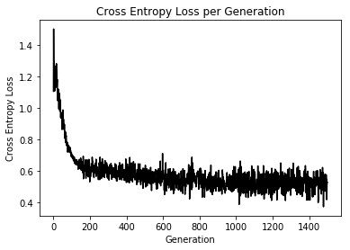
Display model performance

1
2
3
4
5
6
7
8
9
10
11
12
13
14
15
16
%matplotlib inline
# Plot loss over time
plt.plot(loss_vec, 'k-')
plt.title('Cross Entropy Loss per Generation')
plt.xlabel('Generation')
plt.ylabel('Cross Entropy Loss')
plt.show()

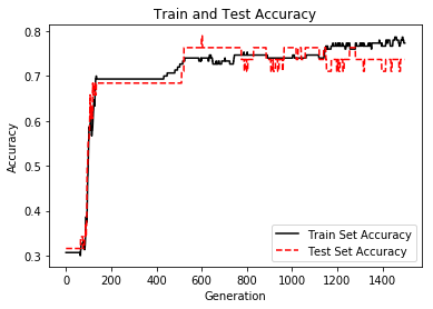
# Plot train and test accuracy
plt.plot(train_acc, 'k-', label='Train Set Accuracy')
plt.plot(test_acc, 'r--', label='Test Set Accuracy')
plt.title('Train and Test Accuracy')
plt.xlabel('Generation')
plt.ylabel('Accuracy')
plt.legend(loc='lower right')
plt.show()

png
png

Learning to Play Tic-Tac-Toe

Tic-Tac-Toe Game
TicTacToeIndexing

Model
TicTacToe Architecture

本站所有文章和源码均免费开放,如您喜欢,可以请我喝杯咖啡