线性回归

Linear Regression (function) https://en.wikipedia.org/wiki/Linear_regression
在现实世界中，存在着大量这样的情况：两个变量例如X和Y有一些依赖关系。由X可以部分地决定Y的值，但这种决定往往不很确切。常常用来说明这种依赖关系的最简单、直观的例子是体重与身高，用Y表示他的体重。众所周知，一般说来，当X大时，Y也倾向于大，但由X不能严格地决定Y。又如，城市生活用电量Y与气温X有很大的关系。在夏天气温很高或冬天气温很低时，由于室内空调、冰箱等家用电器的使用，可能用电就高，相反，在春秋季节气温不高也不低，用电量就可能少。但我们不能由气温X准确地决定用电量Y。类似的例子还很多，变量之间的这种关系称为“相关关系”，回归模型就是研究相关关系的一个有力工具。

Linear Regression

Here we show how to implement various linear regression techniques in TensorFlow. The first two sections show how to do standard matrix linear regression solving in TensorFlow. The remaining six sections depict how to implement various types of regression using computational graphs in TensorFlow.

1. Linear Regression: Inverse Matrix Method

Using the Matrix Inverse Method

Here we implement solving 2D linear regression via the matrix inverse method in TensorFlow.

Model

Given A * x = b, we can solve for x via:

(t(A) A) x = t(A) * b

x = (t(A) A)^(-1) t(A) * b

Here, note that t(A) is the transpose of A.

This script explores how to accomplish linear regression with TensorFlow using the matrix inverse.

Given the system $ A \cdot x = y $, the matrix inverse way of linear regression (equations for overdetermined systems) is given by solving for x as follows.

$x = \left( A^{T} \cdot A \right)^{-1} \cdot A^{T} \cdot y$

As a reminder, here, $x$ is our parameter matrix (vector of length $F+1$, where $F$ is the number of features). Here, $A$, our design matrix takes the form

$A= \begin{bmatrix} 1 & x_{11} & x_{12} & \dots & x_{1F} \\ 1 & x_{21} & x_{22} & \dots & x_{2F} \\ \vdots & \vdots & \vdots & \ddots & \vdots \\ 1 & x_{n1} & x_{n2} & \dots & x_{nF} \end{bmatrix}$

Where $F$ is the number of independent features, and $n$ is the number of points. For an overdetermined system, $n>F$. Remember that one observed point in our system will have length $F+1$ and the $i^{th}$ point will look like

$point_{i} = \left( y_{i}, x_{i1}, x_{i2}, \dots, x_{iF} \right)$

For this recipe, we will consider only a 2-dimensional system ($F=1$), so that we can plot the results at the end.

We start by loading the necessary libraries.

import matplotlib.pyplot as plt
import numpy as np
import tensorflow as tf
from tensorflow.python.framework import ops
ops.reset_default_graph()

Next we start a graph session.

1	sess = tf.Session()

For illustration purposes, we randomly generate data to fit.

The x-values will be a sequence of 100 evenly spaced values between 0 and 100.

The y-values will fit to the line: $y=x$, but we will add normally distributed error according to $N(0,1)$.

1
2
3

# Create the data
x_vals = np.linspace(0, 10, 100)
y_vals = x_vals + np.random.normal(0, 1, 100)

We create the design matrix, $A$, which will be a column of ones and the x-values.

# Create design matrix
x_vals_column = np.transpose(np.matrix(x_vals))
ones_column = np.transpose(np.matrix(np.repeat(1, 100)))
A = np.column_stack((x_vals_column, ones_column))

We now create the y-values as a matrix with Numpy.

After we have the y-values and the design matrix, we create tensors from them.

# Format the y matrix
y = np.transpose(np.matrix(y_vals))

# Create tensors
A_tensor = tf.constant(A)
y_tensor = tf.constant(y)

Now we solve for the parameter matrix with TensorFlow operations.

# Matrix inverse solution
tA_A = tf.matmul(tf.transpose(A_tensor), A_tensor)
tA_A_inv = tf.matrix_inverse(tA_A)
product = tf.matmul(tA_A_inv, tf.transpose(A_tensor))
solution = tf.matmul(product, y_tensor)

Run the solutions and extract the slope and intercept from the parameter matrix.

solution_eval = sess.run(solution)

# Extract coefficients
slope = solution_eval[0][0]
y_intercept = solution_eval[1][0]

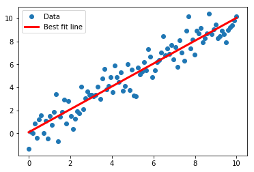
Now we print the solution we found and create a best fit line.

print('slope: ' + str(slope))
print('y_intercept: ' + str(y_intercept))

# Get best fit line
best_fit = []
for i in x_vals:
  best_fit.append(slope*i+y_intercept)

slope: 0.9953458430212332
y_intercept: 0.0956584431188145

We use Matplotlib to plot the results.

# Plot the results
plt.plot(x_vals, y_vals, 'o', label='Data')
plt.plot(x_vals, best_fit, 'r-', label='Best fit line', linewidth=3)
plt.legend(loc='upper left')
plt.show()

2. Linear Regression: Using a Decomposition (Cholesky Method)

Using the Cholesky Decomposition Method

Here we implement solving 2D linear regression via the Cholesky decomposition in TensorFlow.

Model

Given A x = b, and a Cholesky decomposition such that A = LL’ then we can get solve for x via

Solving L y = t(A) b for y
Solving L’ * x = y for x.

This script will use TensorFlow’s function, tf.cholesky() to decompose our design matrix and solve for the parameter matrix from linear regression.

For linear regression we are given the system $A \cdot x = y$. Here, $A$ is our design matrix, $x$ is our parameter matrix (of interest), and $y$ is our target matrix (dependent values).

For a Cholesky decomposition to work we assume that $A$ can be broken up into a product of a lower triangular matrix, $L$ and the transpose of the same matrix, $L^{T}$.

Note that this is when $A$ is square. Of course, with an over determined system, $A$ is not square. So we factor the product $A^{T} \cdot A$ instead. We then assume:

$A^{T} \cdot A = L^{T} \cdot L$

For more information on the Cholesky decomposition and it’s uses, see the following wikipedia link: The Cholesky Decomposition

Given that $A$ has a unique Cholesky decomposition, we can write our linear regression system as the following:

$L^{T} \cdot L \cdot x = A^{T} \cdot y$

Then we break apart the system as follows:

$L^{T} \cdot z = A^{T} \cdot y$

and

$L \cdot x = z$

The steps we will take to solve for $x$ are the following

Compute the Cholesky decomposition of $A$, where $A^{T} \cdot A = L^{T} \cdot L$.
Solve ($L^{T} \cdot z = A^{T} \cdot y$) for $z$.
Finally, solve ($L \cdot x = z$) for $x$.

We start by loading the necessary libraries.

import matplotlib.pyplot as plt
import numpy as np
import tensorflow as tf
from tensorflow.python.framework import ops
ops.reset_default_graph()

Next we create a graph session

1	sess = tf.Session()

We use the same method of generating data as in the prior recipe for consistency.

1
2
3

# Create the data
x_vals = np.linspace(0, 10, 100)
y_vals = x_vals + np.random.normal(0, 1, 100)

We generate the design matrix, $A$.

# Create design matrix
x_vals_column = np.transpose(np.matrix(x_vals))
ones_column = np.transpose(np.matrix(np.repeat(1, 100)))
A = np.column_stack((x_vals_column, ones_column))

Next, we generate the

# Create y matrix
y = np.transpose(np.matrix(y_vals))

# Create tensors
A_tensor = tf.constant(A)
y_tensor = tf.constant(y)

Now we calculate the square of the matrix $A$ and the Cholesky decomposition.

1
2
3

# Find Cholesky Decomposition
tA_A = tf.matmul(tf.transpose(A_tensor), A_tensor)
L = tf.cholesky(tA_A)

We solve the first equation. (see step 2 in the intro paragraph above)

1
2
3

# Solve L*y=t(A)*b
tA_y = tf.matmul(tf.transpose(A_tensor), y)
sol1 = tf.matrix_solve(L, tA_y)

We finally solve for the parameter matrix by solving the second equation (see step 3 in the intro paragraph).

# Solve L' * y = sol1
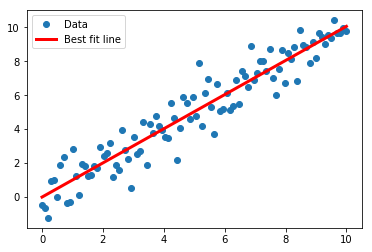
sol2 = tf.matrix_solve(tf.transpose(L), sol1)

solution_eval = sess.run(sol2)

Extract the coefficients and create the best fit line.

# Extract coefficients
slope = solution_eval[0][0]
y_intercept = solution_eval[1][0]

print('slope: ' + str(slope))
print('y_intercept: ' + str(y_intercept))

# Get best fit line
best_fit = []
for i in x_vals:
  best_fit.append(slope*i+y_intercept)

slope: 1.006032728766641
y_intercept: -0.0033007871888138603

Finally, we plot the fit with Matplotlib.

# Plot the results
plt.plot(x_vals, y_vals, 'o', label='Data')
plt.plot(x_vals, best_fit, 'r-', label='Best fit line', linewidth=3)
plt.legend(loc='upper left')
plt.show()

3. Linear Regression: The TensorFlow Way

Learning the TensorFlow Way of Regression

In this section we will implement linear regression as an iterative computational graph in TensorFlow. To make this more pertinent, instead of using generated data, we will instead use the Iris data set. Our x will be the Petal Width, our y will be the Sepal Length. Viewing the data in these two dimensions suggests a linear relationship.

Model

The the output of our model is a 2D linear regression:

y = A * x + b

The x matrix input will be a 2D matrix, where it’s dimensions will be (batch size x 1). The y target output will have the same dimensions, (batch size x 1).

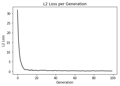
The loss function we will use will be the mean of the batch L2 Loss:

loss = mean( (y_target - model_output)^2 )

We will then iterate through random batch size selections of the data.
For this script, we introduce how to perform linear regression in the context of TensorFlow.

We will solve the linear equation system:

$y = Ax + b$

With the Sepal length (y) and Petal width (x) of the Iris data.

Performing linear regression in TensorFlow is a lot easier than trying to understand Linear Algebra or Matrix decompositions for the prior two recipes. We will do the following:

Create the linear regression computational graph output. This means we will accept an input, $x$, and generate the output, $Ax + b$.
We create a loss function, the L2 loss, and use that output with the learning rate to compute the gradients of the model variables, $A$ and $b$ to minimize the loss.

The benefit of using TensorFlow in this way is that the model can be routinely updated and tweaked with new data incrementally with any reasonable batch size of data. The more iterative we make our machine learning algorithms, the better.

We start by loading the necessary libraries.

import matplotlib.pyplot as plt
import numpy as np
import tensorflow as tf
from sklearn import datasets
from tensorflow.python.framework import ops
ops.reset_default_graph()

We create a graph session.

1	sess = tf.Session()

Next we load the Iris data from the Scikit-Learn library.

# Load the data
# iris.data = [(Sepal Length, Sepal Width, Petal Length, Petal Width)]
iris = datasets.load_iris()
x_vals = np.array([x[3] for x in iris.data])
y_vals = np.array([y[0] for y in iris.data])

With most TensorFlow algorithms, we will need to declare a batch size for the placeholders and operations in the graph. Here, we set it to 25. We can set it to any integer between 1 and the size of the dataset.

For the effect of batch size on the training, see Chapter 2: Batch vs Stochastic Training

1 2	# Declare batch size batch_size = 25

We now initialize the placeholders and variables in the model.

# Initialize placeholders
x_data = tf.placeholder(shape=[None, 1], dtype=tf.float32)
y_target = tf.placeholder(shape=[None, 1], dtype=tf.float32)

# Create variables for linear regression
A = tf.Variable(tf.random_normal(shape=[1,1]))
b = tf.Variable(tf.random_normal(shape=[1,1]))

We add the model operations (linear model output) and the L2 loss.

# Declare model operations
model_output = tf.add(tf.matmul(x_data, A), b)

# Declare loss function (L2 loss)
loss = tf.reduce_mean(tf.square(y_target - model_output))

We have to tell TensorFlow how to optimize and back propagate the gradients. We do this with the standard Gradient Descent operator (tf.train.GradientDescentOptimizer), with the learning rate argument of $0.05$.

Then we initialize all the model variables.

# Declare optimizer
my_opt = tf.train.GradientDescentOptimizer(0.05)
train_step = my_opt.minimize(loss)

# Initialize variables
init = tf.global_variables_initializer()
sess.run(init)

We start our training loop and run the optimizer for 100 iterations.

# Training loop
loss_vec = []
for i in range(100):
    rand_index = np.random.choice(len(x_vals), size=batch_size)
    rand_x = np.transpose([x_vals[rand_index]])
    rand_y = np.transpose([y_vals[rand_index]])
    sess.run(train_step, feed_dict={x_data: rand_x, y_target: rand_y})
    temp_loss = sess.run(loss, feed_dict={x_data: rand_x, y_target: rand_y})
    loss_vec.append(temp_loss)
    if (i+1)%25==0:
        print('Step #' + str(i+1) + ' A = ' + str(sess.run(A)) + ' b = ' + str(sess.run(b)))
        print('Loss = ' + str(temp_loss))

Step #25 A = [[1.5073389]] b = [[3.7461321]]
Loss = 0.53326994
Step #50 A = [[1.2745976]] b = [[4.1358175]]
Loss = 0.42734933
Step #75 A = [[1.1166353]] b = [[4.4049253]]
Loss = 0.29555324
Step #100 A = [[1.0541962]] b = [[4.5658007]]
Loss = 0.23579143

We pull out the optimal coefficients and get the best fit line.

# Get the optimal coefficients
[slope] = sess.run(A)
[y_intercept] = sess.run(b)

# Get best fit line
best_fit = []
for i in x_vals:
  best_fit.append(slope*i+y_intercept)

Plot the results with Matplotlib. Along with the linear fit, we will also plot the L2 loss over the model training iterations.

# Plot the result
plt.plot(x_vals, y_vals, 'o', label='Data Points')
plt.plot(x_vals, best_fit, 'r-', label='Best fit line', linewidth=3)
plt.legend(loc='upper left')
plt.title('Sepal Length vs Petal Width')
plt.xlabel('Petal Width')
plt.ylabel('Sepal Length')
plt.show()

# Plot loss over time
plt.plot(loss_vec, 'k-')
plt.title('L2 Loss per Generation')
plt.xlabel('Generation')
plt.ylabel('L2 Loss')
plt.show()

4. Deming Regression

Model

The model will be the same as regular linear regression:

y = A * x + b

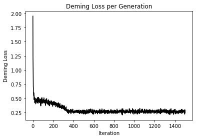
Instead of measuring the vertical L2 distance, we will measure the shortest distance between the line and the predicted point in the loss function.

loss = |y_target - (A * x_input + b)| / sqrt(A^2 + 1)

This function shows how to use TensorFlow to solve linear Deming regression.

$y = Ax + b$

We will use the iris data, specifically:

y = Sepal Length and x = Petal Width.

Deming regression is also called total least squares, in which we minimize the shortest distance from the predicted line and the actual (x,y) points.

If least squares linear regression minimizes the vertical distance to the line, Deming regression minimizes the total distance to the line. This type of regression minimizes the error in the y values and the x values. See the below figure for a comparison.

To implement this in TensorFlow, we start by loading the necessary libraries.

import matplotlib.pyplot as plt
import numpy as np
import tensorflow as tf
from sklearn import datasets
from tensorflow.python.framework import ops
ops.reset_default_graph()

Start a computational graph session:

sess = tf.Session()

# Set a random seed
tf.set_random_seed(42)
np.random.seed(42)

We load the iris data.

# Load the data
# iris.data = [(Sepal Length, Sepal Width, Petal Length, Petal Width)]
iris = datasets.load_iris()
x_vals = np.array([x[3] for x in iris.data]) # Petal Width
y_vals = np.array([y[0] for y in iris.data]) # Sepal Length

Next we declare the batch size, model placeholders, model variables, and model operations.

# Declare batch size
batch_size = 125

# Initialize placeholders
x_data = tf.placeholder(shape=[None, 1], dtype=tf.float32)
y_target = tf.placeholder(shape=[None, 1], dtype=tf.float32)

# Create variables for linear regression
A = tf.Variable(tf.random_normal(shape=[1,1]))
b = tf.Variable(tf.random_normal(shape=[1,1]))

# Declare model operations
model_output = tf.add(tf.matmul(x_data, A), b)

For the demming loss, we want to compute:

$\frac{\left| A \cdot x + b - y \right|}{\sqrt{A^{2} + 1}}$

Which will give us the shortest distance between a point (x,y) and the predicted line, $A \cdot x + b$.

# Declare Deming loss function
deming_numerator = tf.abs(tf.subtract(tf.add(tf.matmul(x_data, A), b), y_target))
deming_denominator = tf.sqrt(tf.add(tf.square(A),1))
loss = tf.reduce_mean(tf.truediv(deming_numerator, deming_denominator))

Next we declare the optimization function and initialize all model variables.

# Declare optimizer
my_opt = tf.train.GradientDescentOptimizer(0.25)
train_step = my_opt.minimize(loss)

# Initialize variables
init = tf.global_variables_initializer()
sess.run(init)

Now we train our Deming regression for 250 iterations.

# Training loop
loss_vec = []
for i in range(1500):
    rand_index = np.random.choice(len(x_vals), size=batch_size)
    rand_x = np.transpose([x_vals[rand_index]])
    rand_y = np.transpose([y_vals[rand_index]])
    sess.run(train_step, feed_dict={x_data: rand_x, y_target: rand_y})
    temp_loss = sess.run(loss, feed_dict={x_data: rand_x, y_target: rand_y})
    loss_vec.append(temp_loss)
    if (i+1)%100==0:
        print('Step #' + str(i+1) + ' A = ' + str(sess.run(A)) + ' b = ' + str(sess.run(b)))
        print('Loss = ' + str(temp_loss))

Step #100 A = [[3.0731559]] b = [[1.7809086]]
Loss = 0.47353575
Step #200 A = [[2.4822469]] b = [[2.522591]]
Loss = 0.41145653
Step #300 A = [[1.7613103]] b = [[3.6220071]]
Loss = 0.37061805
Step #400 A = [[1.0064616]] b = [[4.5484953]]
Loss = 0.26182547
Step #500 A = [[0.9593529]] b = [[4.610097]]
Loss = 0.2435131
Step #600 A = [[0.9646577]] b = [[4.624607]]
Loss = 0.26413646
Step #700 A = [[1.0198785]] b = [[4.6017494]]
Loss = 0.2845798
Step #800 A = [[0.99521935]] b = [[4.6001368]]
Loss = 0.27551532
Step #900 A = [[1.0415721]] b = [[4.6130023]]
Loss = 0.2898117
Step #1000 A = [[1.0065476]] b = [[4.6437864]]
Loss = 0.2525265
Step #1100 A = [[1.0090839]] b = [[4.6393313]]
Loss = 0.27818772
Step #1200 A = [[0.9649767]] b = [[4.581815]]
Loss = 0.25168285
Step #1300 A = [[1.006261]] b = [[4.5881867]]
Loss = 0.25499973
Step #1400 A = [[1.0311592]] b = [[4.618432]]
Loss = 0.2563808
Step #1500 A = [[0.9623312]] b = [[4.5966215]]
Loss = 0.2465789

Retrieve the optimal coefficients (slope and intercept).

# Get the optimal coefficients
[slope] = sess.run(A)
[y_intercept] = sess.run(b)

# Get best fit line
best_fit = []
for i in x_vals:
  best_fit.append(slope*i+y_intercept)

Here is matplotlib code to plot the best fit Deming regression line and the Demming Loss.

# Plot the result
plt.plot(x_vals, y_vals, 'o', label='Data Points')
plt.plot(x_vals, best_fit, 'r-', label='Best fit line', linewidth=3)
plt.legend(loc='upper left')
plt.title('Sepal Length vs Petal Width')
plt.xlabel('Petal Width')
plt.ylabel('Sepal Length')
plt.show()

# Plot loss over time
plt.plot(loss_vec, 'k-')
plt.title('Deming Loss per Generation')
plt.xlabel('Iteration')
plt.ylabel('Deming Loss')
plt.show()

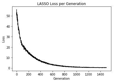
5. LASSO and Ridge Regression

This function shows how to use TensorFlow to solve lasso or ridge regression for $\boldsymbol{y} = \boldsymbol{Ax} + \boldsymbol{b}$

We will use the iris data, specifically: $\boldsymbol{y}$ = Sepal Length, $\boldsymbol{x}$ = Petal Width

# import required libraries
import matplotlib.pyplot as plt
import sys
import numpy as np
import tensorflow as tf
from sklearn import datasets
from tensorflow.python.framework import ops

1 2	# Specify 'Ridge' or 'LASSO' regression_type = 'LASSO'

# clear out old graph
ops.reset_default_graph()

# Create graph
sess = tf.Session()

Load iris data

# iris.data = [(Sepal Length, Sepal Width, Petal Length, Petal Width)]
iris = datasets.load_iris()
x_vals = np.array([x[3] for x in iris.data])
y_vals = np.array([y[0] for y in iris.data])

Model Parameters

# Declare batch size
batch_size = 50

# Initialize placeholders
x_data = tf.placeholder(shape=[None, 1], dtype=tf.float32)
y_target = tf.placeholder(shape=[None, 1], dtype=tf.float32)

# make results reproducible
seed = 13
np.random.seed(seed)
tf.set_random_seed(seed)

# Create variables for linear regression
A = tf.Variable(tf.random_normal(shape=[1,1]))
b = tf.Variable(tf.random_normal(shape=[1,1]))

# Declare model operations
model_output = tf.add(tf.matmul(x_data, A), b)

Loss Functions

# Select appropriate loss function based on regression type

if regression_type == 'LASSO':
    # Declare Lasso loss function
    # Lasso Loss = L2_Loss + heavyside_step,
    # Where heavyside_step ~ 0 if A < constant, otherwise ~ 99
    lasso_param = tf.constant(0.9)
    heavyside_step = tf.truediv(1., tf.add(1., tf.exp(tf.multiply(-50., tf.subtract(A, lasso_param)))))
    regularization_param = tf.multiply(heavyside_step, 99.)
    loss = tf.add(tf.reduce_mean(tf.square(y_target - model_output)), regularization_param)

elif regression_type == 'Ridge':
    # Declare the Ridge loss function
    # Ridge loss = L2_loss + L2 norm of slope
    ridge_param = tf.constant(1.)
    ridge_loss = tf.reduce_mean(tf.square(A))
    loss = tf.expand_dims(tf.add(tf.reduce_mean(tf.square(y_target - model_output)), tf.multiply(ridge_param, ridge_loss)), 0)

else:
    print('Invalid regression_type parameter value',file=sys.stderr)

Optimizer

1
2
3

# Declare optimizer
my_opt = tf.train.GradientDescentOptimizer(0.001)
train_step = my_opt.minimize(loss)

Run regression

# Initialize variables
init = tf.global_variables_initializer()
sess.run(init)

# Training loop
loss_vec = []
for i in range(1500):
    rand_index = np.random.choice(len(x_vals), size=batch_size)
    rand_x = np.transpose([x_vals[rand_index]])
    rand_y = np.transpose([y_vals[rand_index]])
    sess.run(train_step, feed_dict={x_data: rand_x, y_target: rand_y})
    temp_loss = sess.run(loss, feed_dict={x_data: rand_x, y_target: rand_y})
    loss_vec.append(temp_loss[0])
    if (i+1)%300==0:
        print('Step #' + str(i+1) + ' A = ' + str(sess.run(A)) + ' b = ' + str(sess.run(b)))
        print('Loss = ' + str(temp_loss))
        print('\n')

Step #300 A = [[0.7717163]] b = [[1.8247688]]
Loss = [[10.26617]]


Step #600 A = [[0.75910366]] b = [[3.2217226]]
Loss = [[3.059304]]


Step #900 A = [[0.74844867]] b = [[3.9971633]]
Loss = [[1.2329929]]


Step #1200 A = [[0.73754]] b = [[4.429276]]
Loss = [[0.57923675]]


Step #1500 A = [[0.72945035]] b = [[4.672014]]
Loss = [[0.40877518]]

Extract regression results

# Get the optimal coefficients
[slope] = sess.run(A)
[y_intercept] = sess.run(b)

# Get best fit line
best_fit = []
for i in x_vals:
  best_fit.append(slope*i+y_intercept)

Plot results

%matplotlib inline
# Plot the result
plt.plot(x_vals, y_vals, 'o', label='Data Points')
plt.plot(x_vals, best_fit, 'r-', label='Best fit line', linewidth=3)
plt.legend(loc='upper left')
plt.title('Sepal Length vs Pedal Width')
plt.xlabel('Pedal Width')
plt.ylabel('Sepal Length')
plt.show()

# Plot loss over time
plt.plot(loss_vec, 'k-')
plt.title(regression_type + ' Loss per Generation')
plt.xlabel('Generation')
plt.ylabel('Loss')
plt.show()

6. Elastic Net Regression

This function shows how to use TensorFlow to solve elastic net regression.
$y = Ax + b$

Setup model

# make results reproducible
seed = 13
np.random.seed(seed)
tf.set_random_seed(seed)

# Declare batch size
batch_size = 50

# Initialize placeholders
x_data = tf.placeholder(shape=[None, 3], dtype=tf.float32)
y_target = tf.placeholder(shape=[None, 1], dtype=tf.float32)

# Create variables for linear regression
A = tf.Variable(tf.random_normal(shape=[3,1]))
b = tf.Variable(tf.random_normal(shape=[1,1]))

# Declare model operations
model_output = tf.add(tf.matmul(x_data, A), b)

# Declare the elastic net loss function
elastic_param1 = tf.constant(1.)
elastic_param2 = tf.constant(1.)
l1_a_loss = tf.reduce_mean(tf.abs(A))
l2_a_loss = tf.reduce_mean(tf.square(A))
e1_term = tf.multiply(elastic_param1, l1_a_loss)
e2_term = tf.multiply(elastic_param2, l2_a_loss)
loss = tf.expand_dims(tf.add(tf.add(tf.reduce_mean(tf.square(y_target - model_output)), e1_term), e2_term), 0)

# Declare optimizer
my_opt = tf.train.GradientDescentOptimizer(0.001)
train_step = my_opt.minimize(loss)

7. Logistic Regression

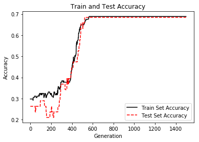
Implementing Logistic Regression

Logistic regression is a way to predict a number between zero or one (usually we consider the output a probability). This prediction is classified into class value ‘1’ if the prediction is above a specified cut off value and class ‘0’ otherwise. The standard cutoff is 0.5. For the purpose of this example, we will specify that cut off to be 0.5, which will make the classification as simple as rounding the output.

The data we will use for this example will be the UMASS low birth weight data.

Model

The the output of our model is the standard logistic regression:

y = sigmoid(A * x + b)

The x matrix input will have dimensions (batch size x # features). The y target output will have the dimension batch size x 1.

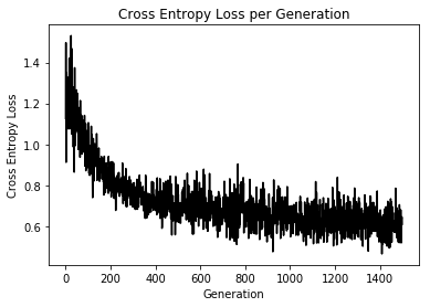
The loss function we will use will be the mean of the cross-entropy loss:

loss = mean( - y log(predicted) + (1-y) log(1-predicted) )

TensorFlow has this cross entropy built in, and we can use the function, ‘tf.nn.sigmoid_cross_entropy_with_logits()’

We will then iterate through random batch size selections of the data.

This function shows how to use TensorFlow to solve logistic regression.
$ \textbf{y} = sigmoid(\textbf{A}\times \textbf{x} + \textbf{b})$

We will use the low birth weight data, specifically:

1 2	# y = 0 or 1 = low birth weight # x = demographic and medical history data

import matplotlib.pyplot as plt
import numpy as np
import tensorflow as tf
import requests
from tensorflow.python.framework import ops
import os.path
import csv

ops.reset_default_graph()

# Create graph
sess = tf.Session()

Obtain and prepare data for modeling

# name of data file
birth_weight_file = 'birth_weight.csv'

# download data and create data file if file does not exist in current directory
if not os.path.exists(birth_weight_file):

    birthdata_url = 'https://github.com/nfmcclure/tensorflow_cookbook/' + \
    'raw/master/01_Introduction/07_Working_with_Data_Sources/birthweight_data/birthweight.dat'
    birth_file = requests.get(birthdata_url)
    birth_data = birth_file.text.split('\r\n')
    birth_header = birth_data[0].split('\t')
    birth_data = [[float(x) for x in y.split('\t') if len(x)>=1] for y in birth_data[1:] if len(y)>=1]
    with open(birth_weight_file, 'w', newline='') as f:
        writer = csv.writer(f)
        writer.writerow(birth_header)
        writer.writerows(birth_data)
        f.close()

# read birth weight data into memory
birth_data = []
with open(birth_weight_file, newline='') as csvfile:
     csv_reader = csv.reader(csvfile)
     birth_header = next(csv_reader)
     for row in csv_reader:
         birth_data.append(row)

birth_data = [[float(x) for x in row] for row in birth_data]

# Pull out target variable
y_vals = np.array([x[0] for x in birth_data])
# Pull out predictor variables (not id, not target, and not birthweight)
x_vals = np.array([x[1:8] for x in birth_data])

# set for reproducible results
seed = 99
np.random.seed(seed)
tf.set_random_seed(seed)

# Split data into train/test = 80%/20%
train_indices = np.random.choice(len(x_vals), round(len(x_vals)*0.8), replace=False)
test_indices = np.array(list(set(range(len(x_vals))) - set(train_indices)))
x_vals_train = x_vals[train_indices]
x_vals_test = x_vals[test_indices]
y_vals_train = y_vals[train_indices]
y_vals_test = y_vals[test_indices]

# Normalize by column (min-max norm)
def normalize_cols(m, col_min=np.array([None]), col_max=np.array([None])):
    if not col_min[0]:
        col_min = m.min(axis=0)
    if not col_max[0]:
        col_max = m.max(axis=0)
    return (m-col_min) / (col_max - col_min), col_min, col_max

x_vals_train, train_min, train_max = np.nan_to_num(normalize_cols(x_vals_train))
x_vals_test, _, _ = np.nan_to_num(normalize_cols(x_vals_test, train_min, train_max))

Define Tensorflow computational graph

# Declare batch size
batch_size = 25

# Initialize placeholders
x_data = tf.placeholder(shape=[None, 7], dtype=tf.float32)
y_target = tf.placeholder(shape=[None, 1], dtype=tf.float32)

# Create variables for linear regression
A = tf.Variable(tf.random_normal(shape=[7,1]))
b = tf.Variable(tf.random_normal(shape=[1,1]))

# Declare model operations
model_output = tf.add(tf.matmul(x_data, A), b)

# Declare loss function (Cross Entropy loss)
loss = tf.reduce_mean(tf.nn.sigmoid_cross_entropy_with_logits(logits=model_output, labels=y_target))

# Declare optimizer
my_opt = tf.train.GradientDescentOptimizer(0.01)
train_step = my_opt.minimize(loss)

Train model

# Initialize variables
init = tf.global_variables_initializer()
sess.run(init)

# Actual Prediction
prediction = tf.round(tf.sigmoid(model_output))
predictions_correct = tf.cast(tf.equal(prediction, y_target), tf.float32)
accuracy = tf.reduce_mean(predictions_correct)

# Training loop
loss_vec = []
train_acc = []
test_acc = []
for i in range(1500):
    rand_index = np.random.choice(len(x_vals_train), size=batch_size)
    rand_x = x_vals_train[rand_index]
    rand_y = np.transpose([y_vals_train[rand_index]])
    sess.run(train_step, feed_dict={x_data: rand_x, y_target: rand_y})

    temp_loss = sess.run(loss, feed_dict={x_data: rand_x, y_target: rand_y})
    loss_vec.append(temp_loss)
    temp_acc_train = sess.run(accuracy, feed_dict={x_data: x_vals_train, y_target: np.transpose([y_vals_train])})
    train_acc.append(temp_acc_train)
    temp_acc_test = sess.run(accuracy, feed_dict={x_data: x_vals_test, y_target: np.transpose([y_vals_test])})
    test_acc.append(temp_acc_test)
    if (i+1)%300==0:
        print('Loss = ' + str(temp_loss))

Loss = 0.6944471
Loss = 0.7304496
Loss = 0.62496805
Loss = 0.69695
Loss = 0.6096429

Display model performance

%matplotlib inline
# Plot loss over time
plt.plot(loss_vec, 'k-')
plt.title('Cross Entropy Loss per Generation')
plt.xlabel('Generation')
plt.ylabel('Cross Entropy Loss')
plt.show()

# Plot train and test accuracy
plt.plot(train_acc, 'k-', label='Train Set Accuracy')
plt.plot(test_acc, 'r--', label='Test Set Accuracy')
plt.title('Train and Test Accuracy')
plt.xlabel('Generation')
plt.ylabel('Accuracy')
plt.legend(loc='lower right')
plt.show()